
A to Z of Excel Functions: The MAKEARRAY Function
13 December 2021
Welcome back to our regular A to Z of Excel Functions blog. Today we look at the MAKEARRAY function.
The MAKEARRAY function
MAKEARRAY returns a calculated array of a specified row and column size, by applying a LAMBDA function. This function is useful for situations where you wish to combine or transform arrays, as well as being useful for generating data. The syntax is as follows:
MAKEARRAY(rows, columns, lambda)
It has the following arguments:
- rows: this argument is required and represents the number of rows in the array (which must be greater than zero)
- columns: this argument is also required and represents the number of columns in the array (which again must be greater than zero)
- lambda: also necessary, this is the LAMBDA that is called to create the array. In particular, this lambda function must take two parameters, namely:
- row_index: the index of the row (row number)
- column_index: the index of the column (column number).
As an example, consider the following:
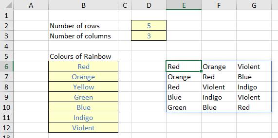
Imagine, for reasons best known to myself, I wanted to generate an array of colours of the rainbow (albeit with the final colour, ahem, slightly amended). In the image above, I have specified the number of rows (cell D2) and the number of columns (cell D3) in my array, and listed the colours in cells B6:B12 inclusive.
The formula in cell E6 is given by
=MAKEARRAY(D2, D3, LAMBDA(row, column, INDEX(B6:B12, RANDBETWEEN(1, 7))))
The first two arguments in this formula are D2 and D3, which refer to the number of rows and columns for the array to be generated respectively. The final argument of MAKEARRAY is the LAMBDA, which must take two parameters, corresponding to the value generated by LAMBDA, namely:
- row: the index of the row
- column: the index of the column.
The calculation thus uses the non-dynamic array function RANDBETWEEN to generate an integer between one [1] and seven [7] to select from the list of colours of the rainbow, stipulated in cells B6:B12. For example, if Excel generates the number 5, the value “Blue” will be chosen, etc.
Now it is true that existing functions could be used to achieve the same result, e.g.
=INDEX(B6:B12, RANDARRAY(D2, D3, 1, 7, TRUE))
This formula seems shorter and simpler, and indeed, may be the better option for this above illustration. But that is exactly what this is – a simple example. As more complex arrays need to be created, existing function counterparts may prove difficult, convoluted or impossible to construct – and this is precisely where MAKEARRAY and LAMBDA come in.
We’ll continue our A to Z of Excel Functions soon. Keep checking back – there’s a new blog post every other business day.
A full page of the function articles can be found here.