
Charts and Dashboards: The Point and Figure Chart – Part 2
21 July 2023
Welcome back to our Charts and Dashboards blog series. This week, we continue to explain how to create a bespoke Point and Figure chart by looking at how we use the summary data to prepare the chart data.
Prepare Data
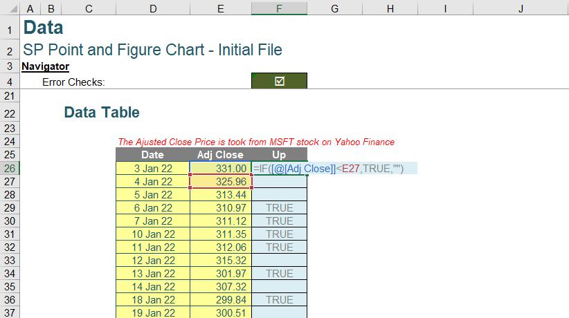
To prepare the data, the first step is to calculate the data in the Data Table. This involves creating a new column called Up where a formula is entered to determine every time the stock price goes up. The formula used is:
=IF([@[Adj Close]]<E26,TRUE,"")
This formula compares the current price and the next day’s price. If the current price is higher, it will leave the cell blank; otherwise, it will return TRUE.
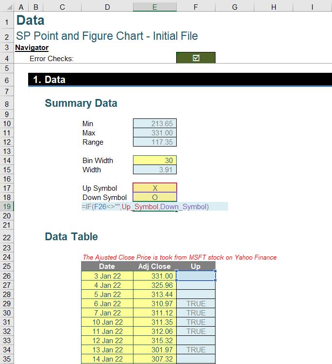
After creating the Up column, the next step is to finish the Starting_Symbol cell. This is done by writing a formula to determine which symbol goes first. The formula used is:
=IF(F25<>"",Up_Symbol,Down_Symbol)
If the first cell of the Data Table is empty, it means the stock price is falling, and if it is not empty, it means the stock price is rising.
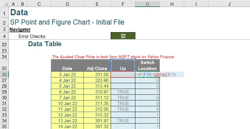
Next, a new column called Switch Location is created to track the point where the stock price has a reversal movement. The formula used is:
=IF(F24=[@Up],0,1)
The F24 cell is in the Up column and is one cell above the current Up cell. This formula keeps track of any difference in the Up column between the current and previous date. If both cells in Up column do not equal each other, a value of one [1] is put there to signal the turning point of the stock price. If they are equal, a value of zero [0] is put there to signal that there is no change in direction. The starting date of the analysis always counts as one turning point in the stock price, forcing the indexing in later step to always start from one [1].
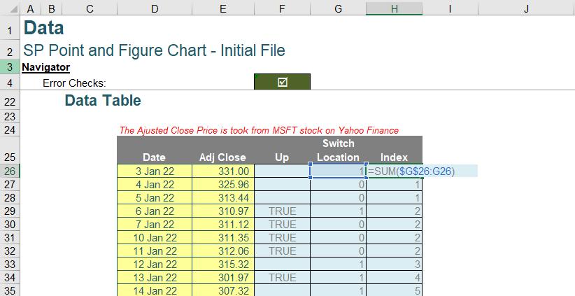
The next column needed is the Index column, which assigns the index group for each price movement. Ideally, if a stock price never has down movements in their price, the Index column should be filled with one [1] from top to bottom. The formula used for this column is a cumulative sum of the "Switch Location" column:
=SUM($G$26:G26)
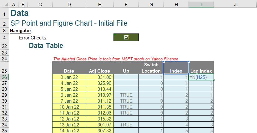
Finally, the last column needed for the table is Lag Index. As the name suggests, this column takes the index of the previous or prior as its value. The reason for this is that the Index column will not include the value of the turning point at the end of the stock price direction. Hence, a Lag Index is needed to recapture that with the following formula:
=N(H25)
Next time, we will Transform the data.
That’s it for this week. Check back next week for more Charts and Dashboards tips.