
Monday Morning Mulling: March 2022 Challenge
28 March 2022
On the final Friday of each month, we set an Excel / Power Pivot / Power Query / Power BI problem for you to puzzle over for the weekend. On the Monday, we publish a solution. If you think there is an alternative answer, feel free to email us. We’ll feel free to ignore you.
The challenge this month was to create a formula for finding first visible cell in a range. Easy, yes?
The Challenge

In this challenge, we required you to create a formula for finding first visible cell in a filtered range without using VBA and macros.
You can download the question file here.
As always, there was a requirement:
- this was a formula challenge; no Power Query / Get & Transform or VBA!
Suggested Solutions
You can find our Excel file here which demonstrates our suggested solutions. However, before explaining our solutions, we will clarify the common idea how we came up with them first.
For Excel Office 365, Excel on the Web and Office Beta / Insider versions:
These Excel versions allow us to use Dynamic Arrays which help shorten a lot of steps.
To begin with, we can generate a new column using SUBTOTAL function which comes up with subtotal in given list or database. Do not forget to use the COUNTA function in SUBTOTAL function as the given data consists of text.
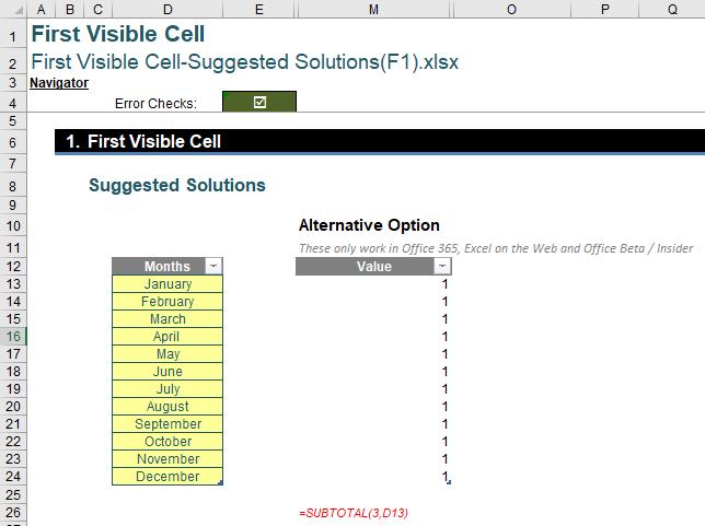
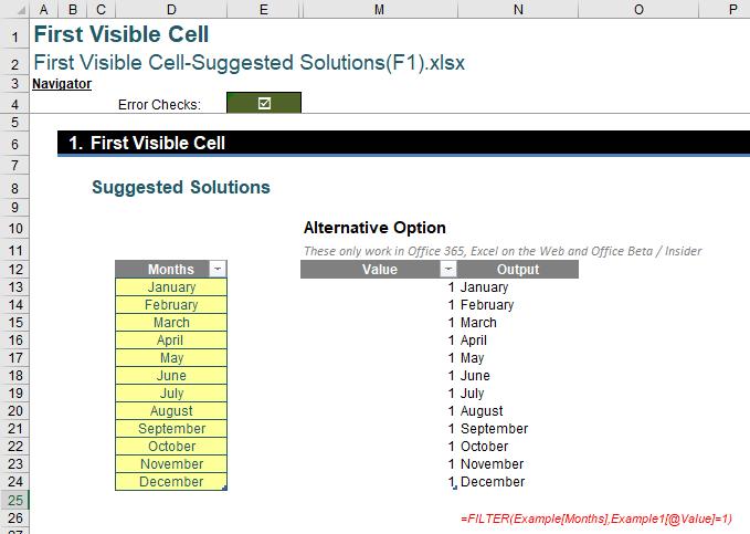
Finally, the FILTER function of dynamic arrays is used in order to find the first visible cell in each range and using the following formula:
=FILTER(Example[Months],Example1[@Value]=1)
The resulting list will be spilled range created by the formula above written in only cell N13 as below:
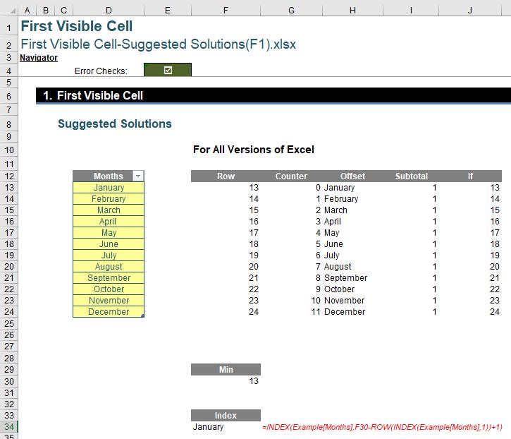
For all current Excel versions:
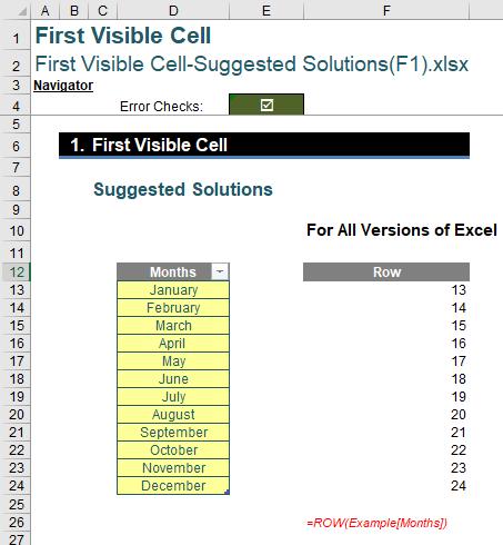
As there is no FILTER function (i.e. Dynamic Array functions) in other Excel versions, firstly we need to create a few helper columns. To begin with we will be using the ROW function in order to find out the row number of the given data by:
=ROW(Example[Months])
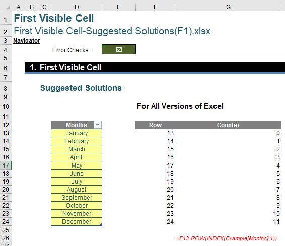
Then, the next step would be to find out the counter number for each month through:
=F13-ROW(INDEX(Example[Months],1))
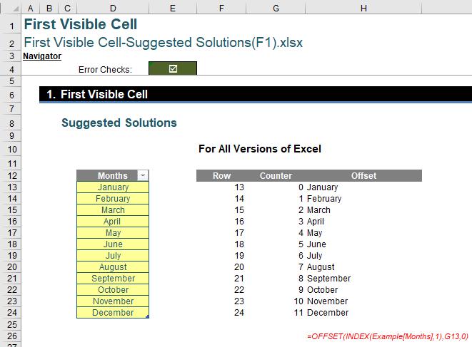
The next step would be to use INDEX function inside OFFSET function in order to find out the given month for each counter number using :
=OFFSET(INDEX(Example[Months],1),G13,0)
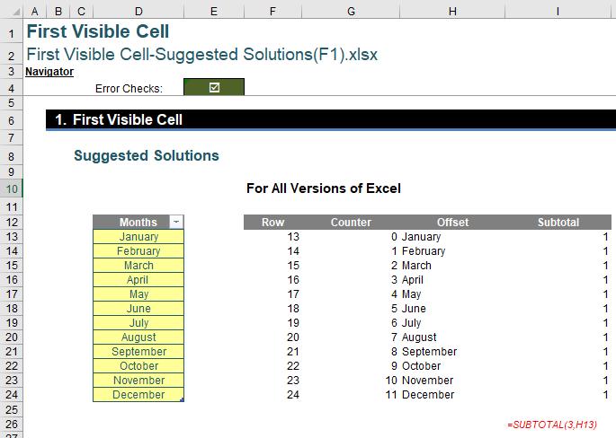
Next step would be to use the COUNTA function inside SUBTOTAL in order to count visible text on each row of 'Offset' column by:
=SUBTOTAL(3,H13)
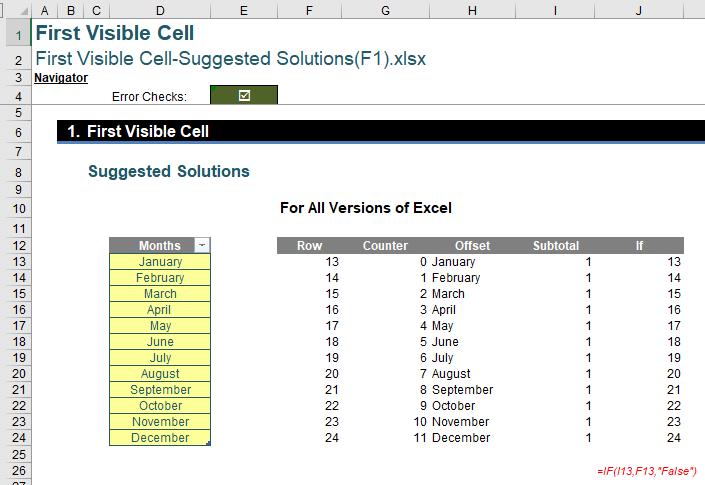
Then, we can use IF function in order to return the row number against the 'Subtotal' column using:
=IF(I13,F13,”False”)
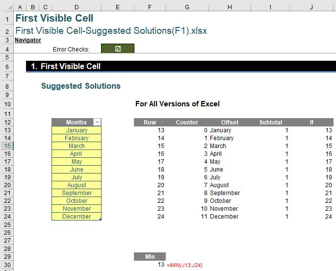
The next step is to find out row number of the first visible cell using MIN formula for 'If' column:
=MIN(J13:J24)
The final step would be to use INDEX function in order to find out the first visible cell in the given range by:
=INDEX(Example[Months],F30-ROW(INDEX(Example[Months],1))+1)
Full formula:
=INDEX(Example[Months], MIN(IF(SUBTOTAL(3,OFFSET(INDEX(Example[Months],1),ROW(Example[Months])-ROW(INDEX(Example[Months],1)),0)),ROW(Example[Months])-ROW(INDEX(Example[Months],1))+1)))
The Final Friday Fix will return on Friday 29 April 2022 with a new Excel Challenge. In the meantime, please look out for the Daily Excel Tip on our home page and watch out for a new blog every business working day.