
Power Pivot Principles: Lookups in Power Pivot
18 December 2018
Welcome back to our Power Pivot blog. Today, we discuss how to create lookups in Power Pivot.
The ability to create lookup columns in Excel is very useful, especially when we have a table that only contains an identifier of some sort but the data we need, such as the product name, is stored elsewhere.
For example, let’s assume that we have the following table that contains today’s (at the time of writing) shipment:
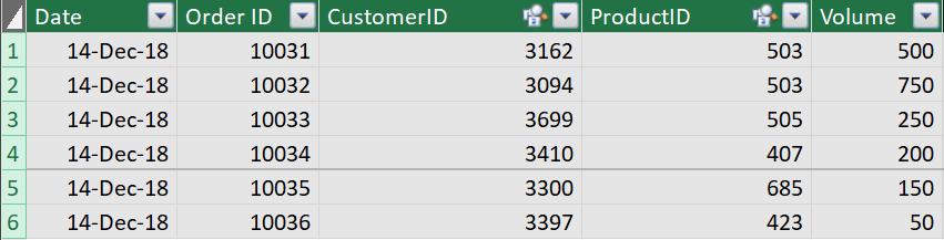
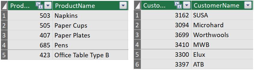
Yes, the table is useful however the table only contains the Product ID and Customer ID, making this particularly difficult to read for humans. The customer and product names are stored in other (related) tables, viz.
We can use the RELATED function to create two custom columns in the shipment table that will display the Product Name and Customer Name. You should note that before creating the custom columns, ensure that the three tables have been loaded to the data model and have established relationships between them (you can read more about establishing relationships between tables here).

To create our custom columns, navigate to the Power Pivot window and create a custom column on our Shipping Table (you can read more about creating custom columns here):

It’s simple:
=RELATED(‘Customer Table’[CustomerName]).
We add another column for the Product Name:
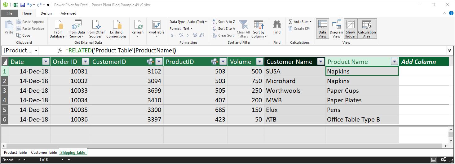
=RELATED(‘Product Table’[ProductName]).
There we have it, using the RELATED function we have created a much more readable table.
That’s it for this week, happy pivoting!
Stay tuned for our next post on Power Pivot in the Blog section. In the meantime, please remember we have training in Power Pivot which you can find out more about here. If you wish to catch up on past articles in the meantime, you can find all of our Past Power Pivot blogs here.