Power Query: Candid Columns

Welcome to our Power Query blog. This week, I look at an example where data comes in one Excel column and needs to be converted to a table.

Not all data arrives in Excel in nicely organised tables. John the imaginary salesperson has sent in some new contacts, which he has copied to a worksheet:

I have a list of names and addresses in a column.  I would like them to be in a table, where I can extract the name, address, country and post code (aka zip code).  I start by creating a new query from my data using the ‘From Table’ option in the ‘Get & Transform’ section on the ‘Data’ tab.

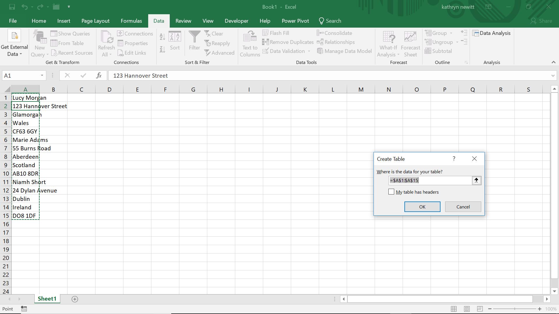
Power Query asks me to confirm where my table is, and whether it has headers (no, thanks to John, it doesn’t!). The default looks fine so I click ‘OK’.

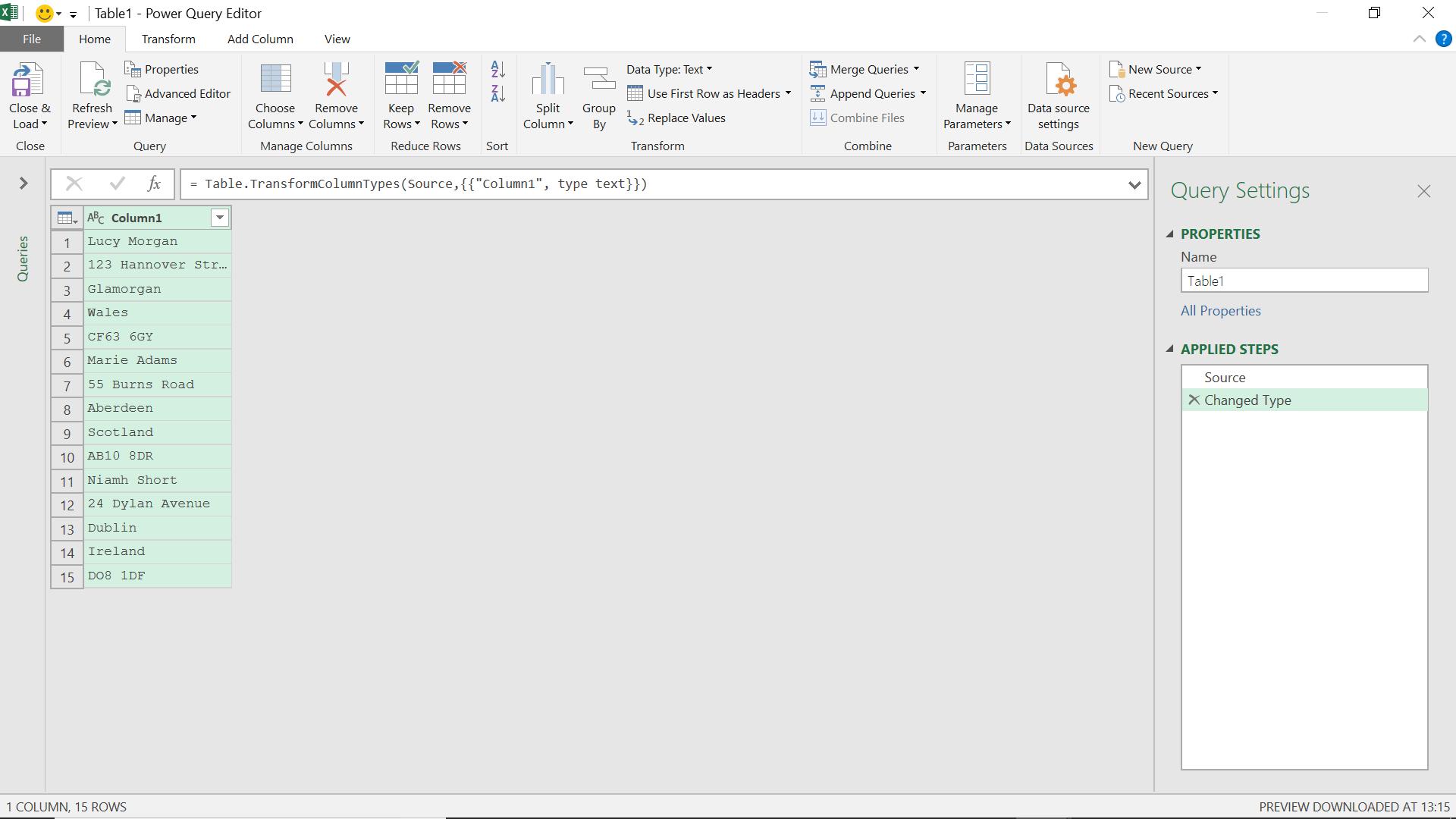
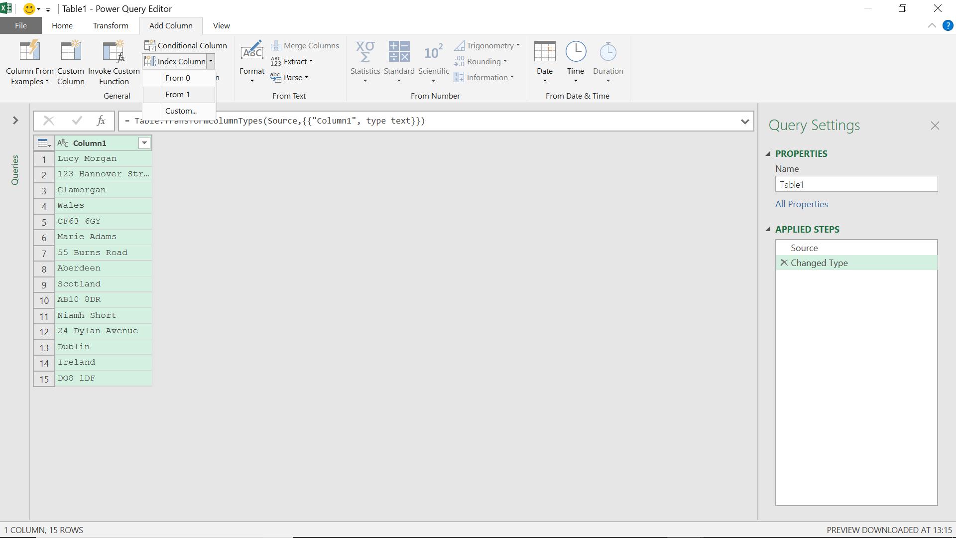
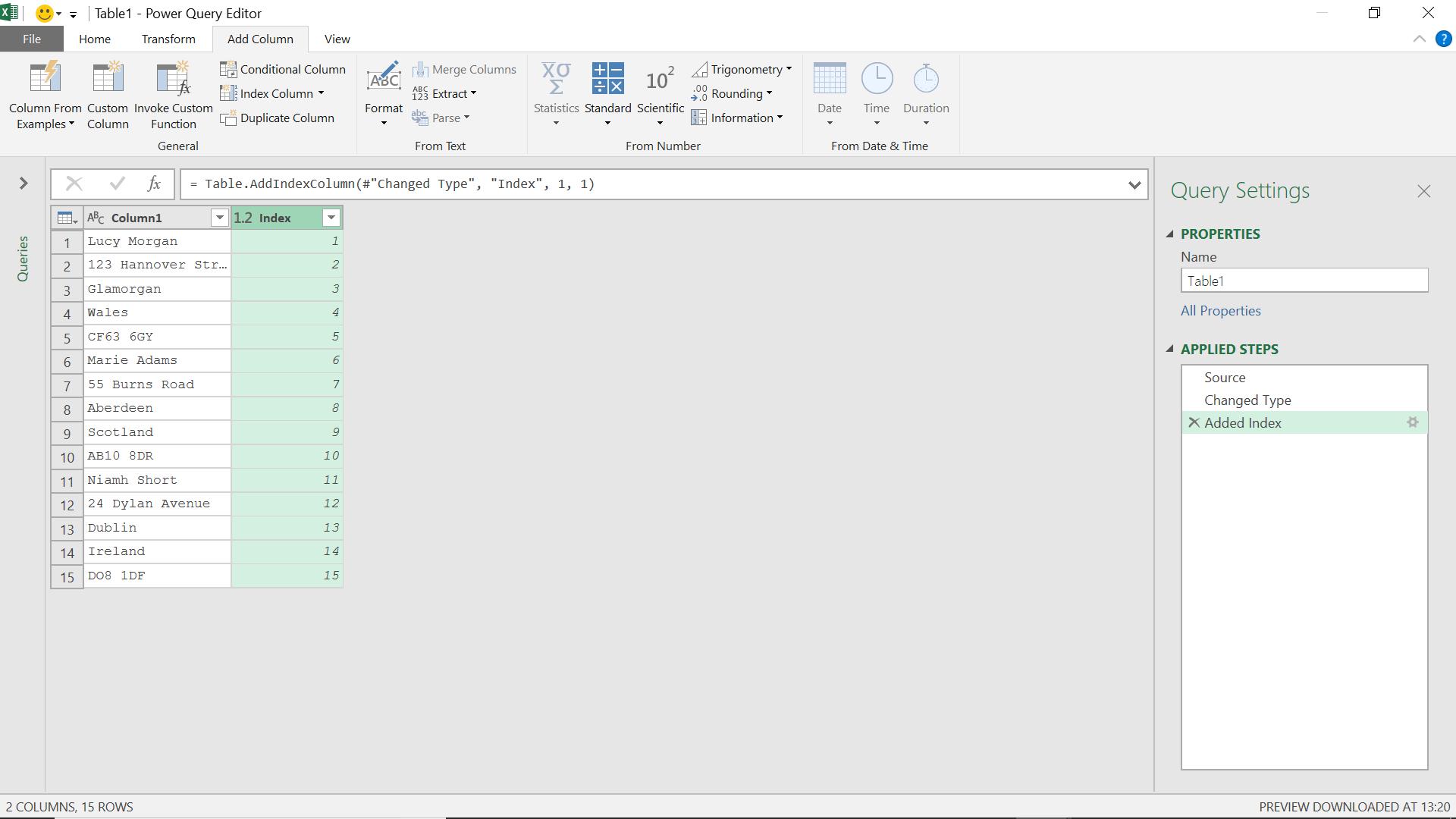
My data is extracted, and now I can set about transforming it into a useful table. Since my data is grouped into five rows for each address (and in this case I can rely on this being consistent because it comes from a database which ensures this), it would be useful to count which row I am on. I can do this by creating an index column. In the ‘Add Column’ tab, I choose ‘Index Column’ in the ‘General’ section, and start my column from 1.

Having created my column I now have some mathematical possibilities.

I am going to use the function Number.Mod() to determine where each address starts.  Number.Mod() divides one number by another number and gives the remainder.  This is similar to the MOD function in Excel. 

It’s much clearer to see it in practice.  To see where each address starts, I divide the index by five and look at the remainder.  I create a new ‘Custom Column’ viz.

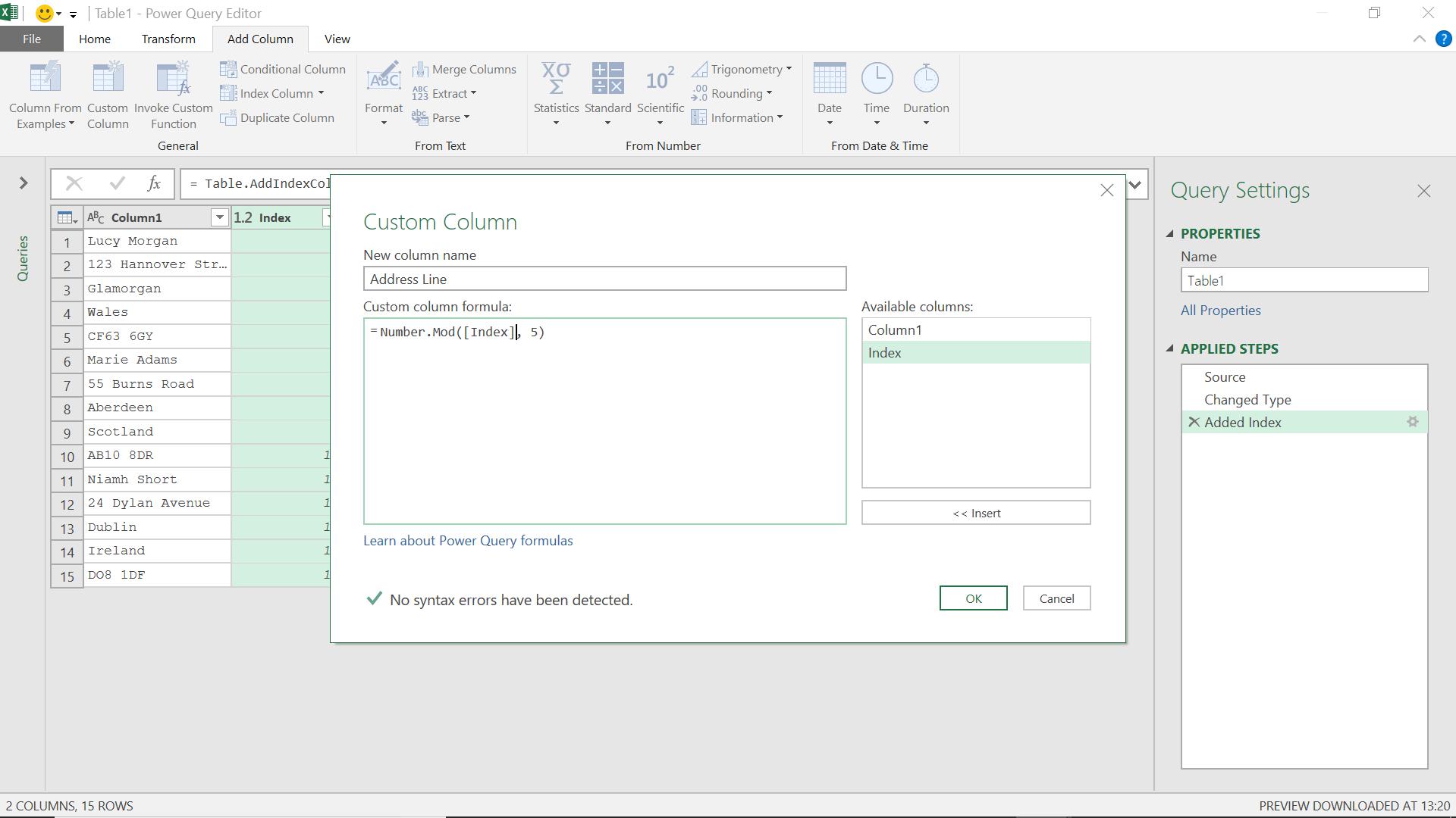
I click ‘OK’ to create my new column.

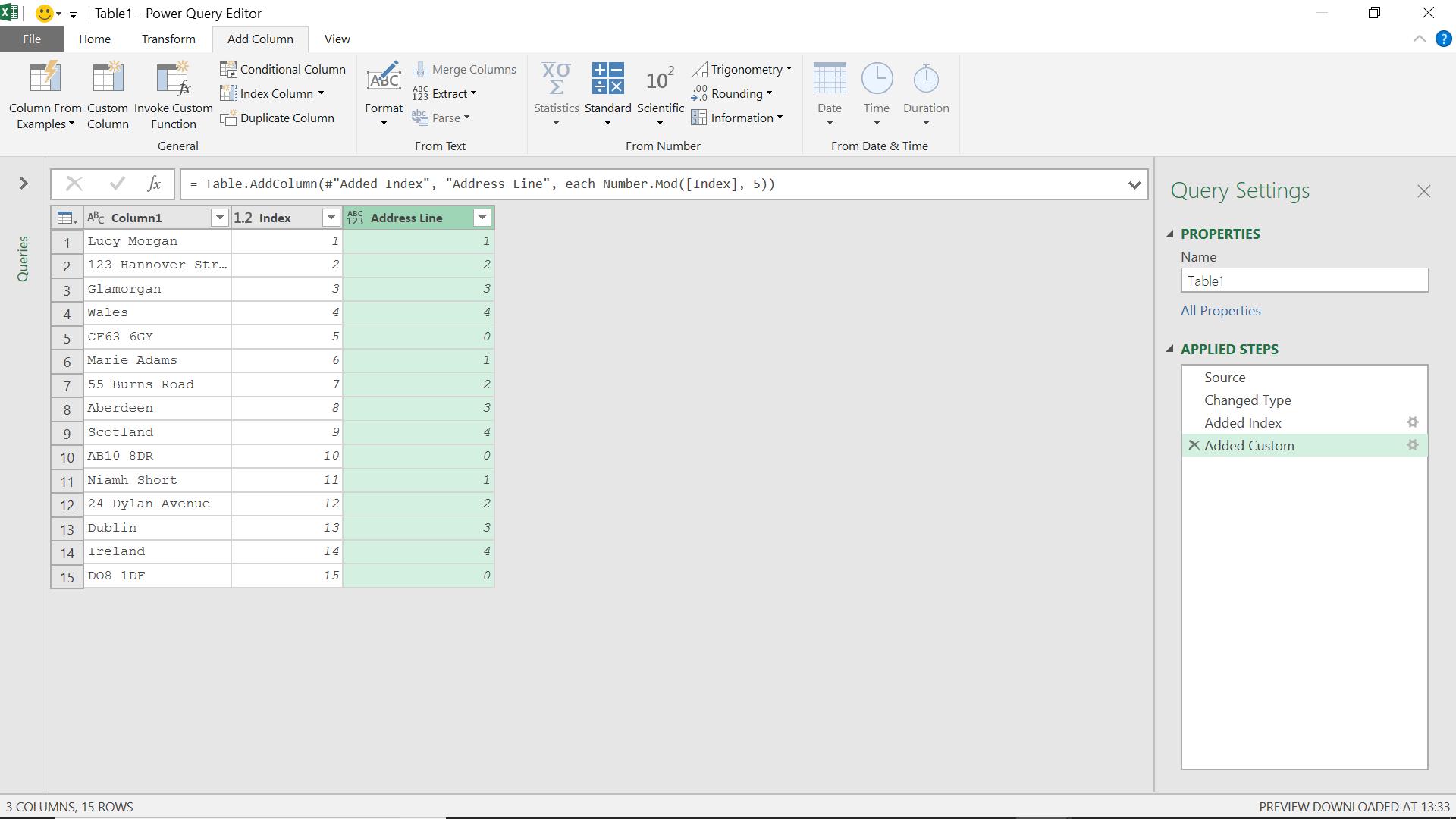
My aim is to indicate which address lines belong together, by giving them the same value. I am going to do this with a running total (for more details on how to create a running total, please see Power Query: One Route to a Running Total.

My first step is to only count at the beginning of each address, and to do this I create another column, which this time is a ‘Conditional Column’:

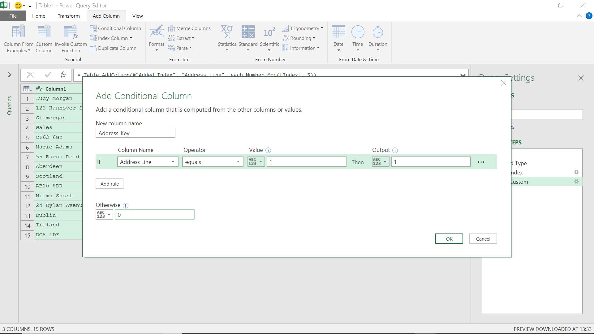
This column will be 1 for the first line and zero for the rest.

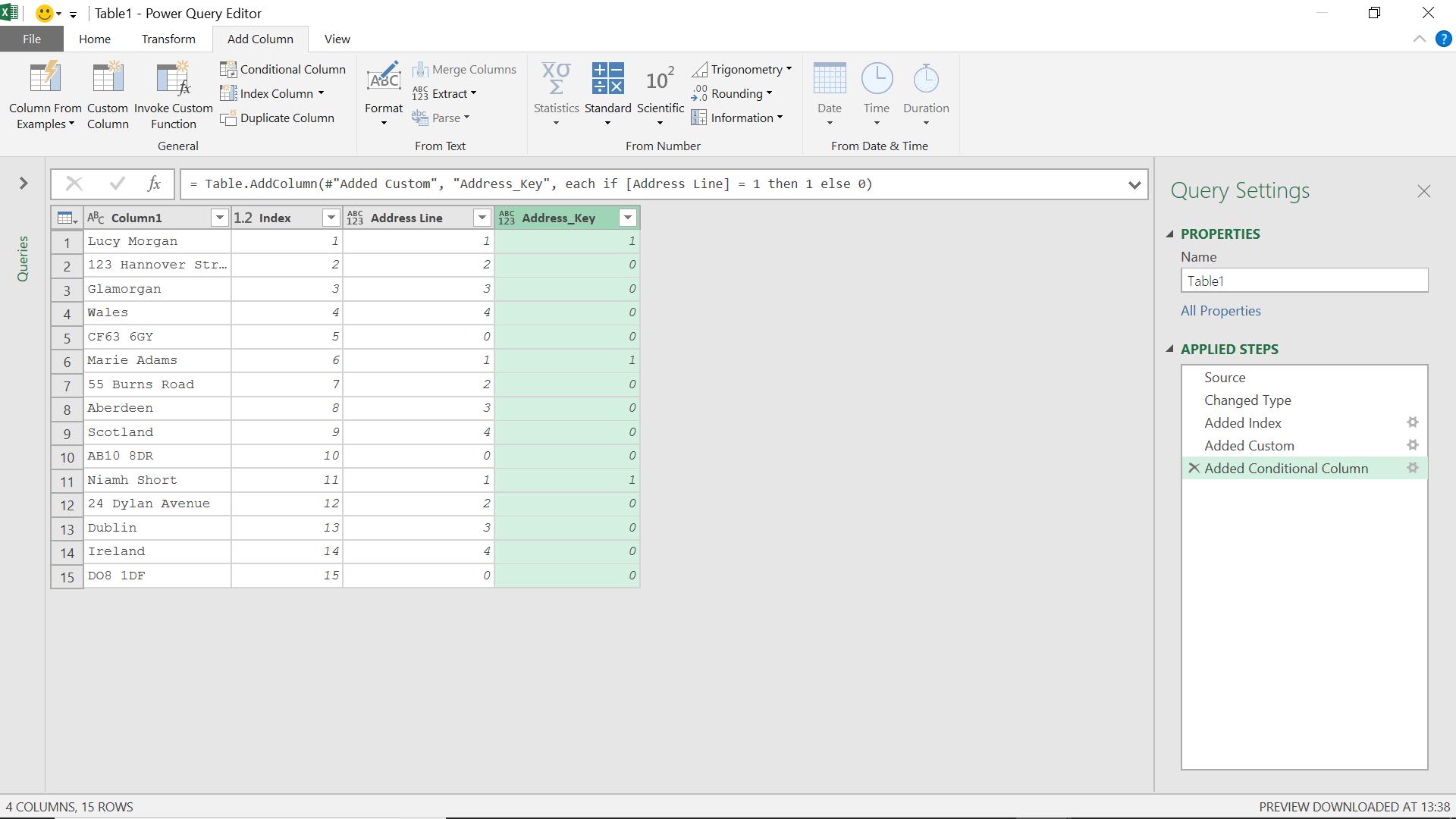
I can now create another ‘Custom Column’ for my running total.

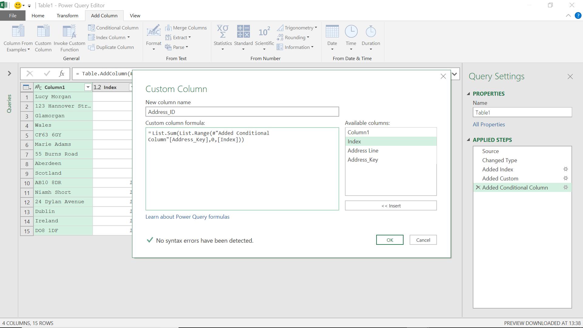
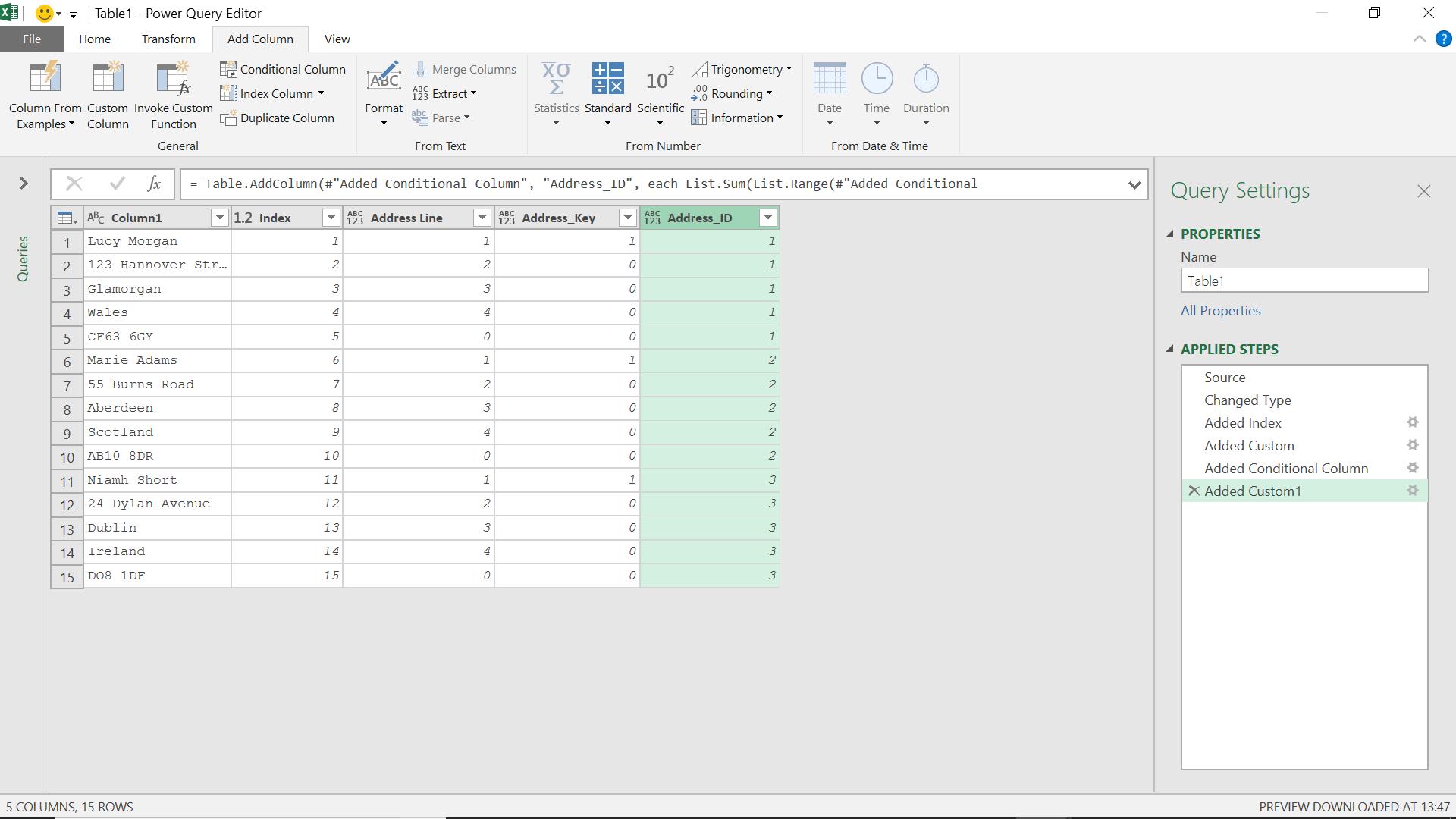
This gives me the same value for each line belonging to the same address.

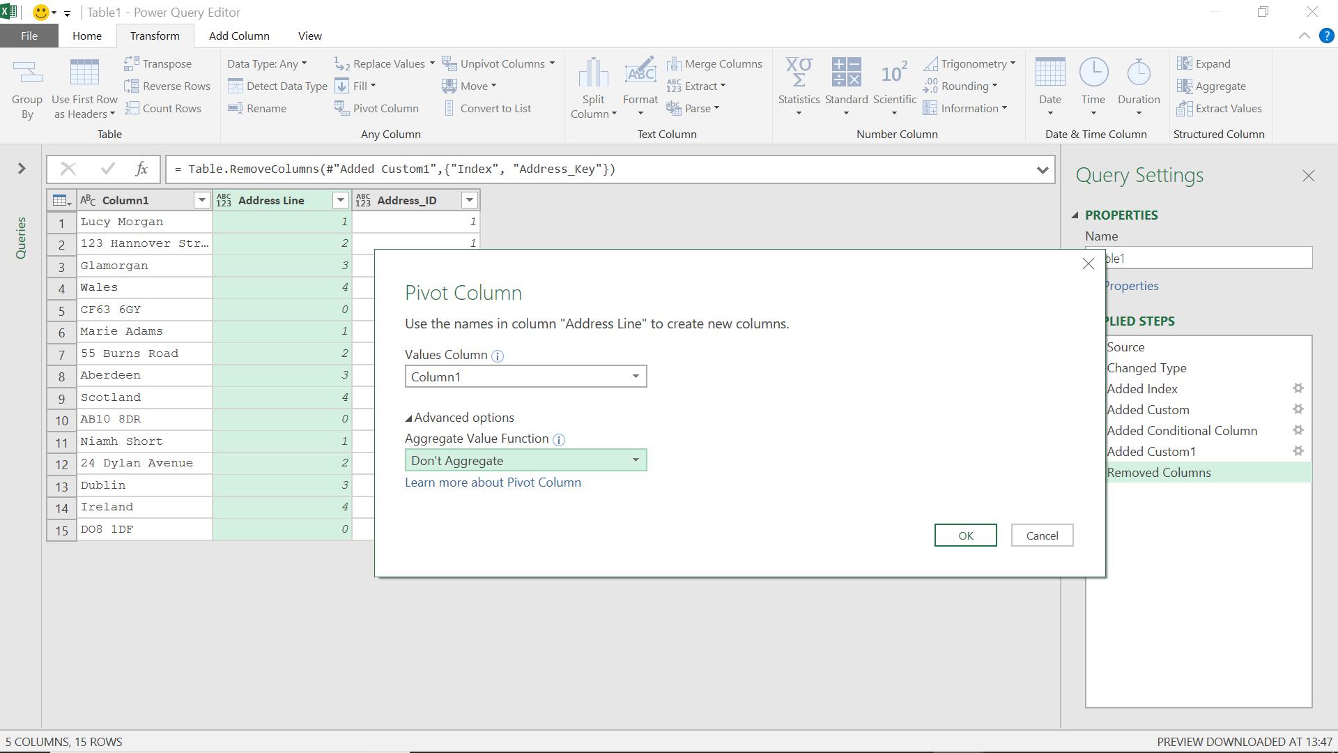
Now I have a way to identify each address, I am ready to pivot my data. I no longer need my index or Address_Key columns, so I can remove these first.

On the ‘Transform’ tab I select Address_Line and choose to pivot my data. The values will be in Column1 and I don’t want to aggregate.

I click ‘OK’ to see my data.

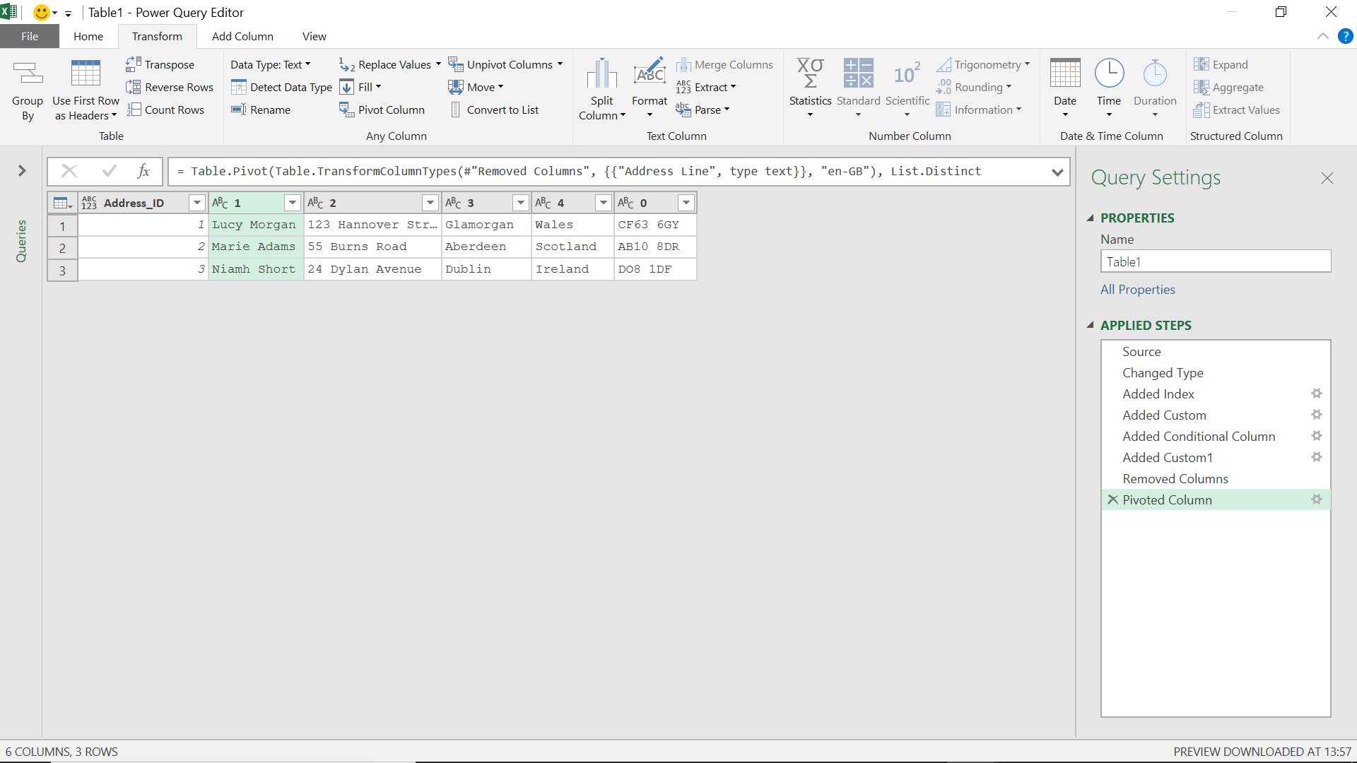
This is looking much better. My Address_ID column is populated correctly, so I just need to rename my other columns.

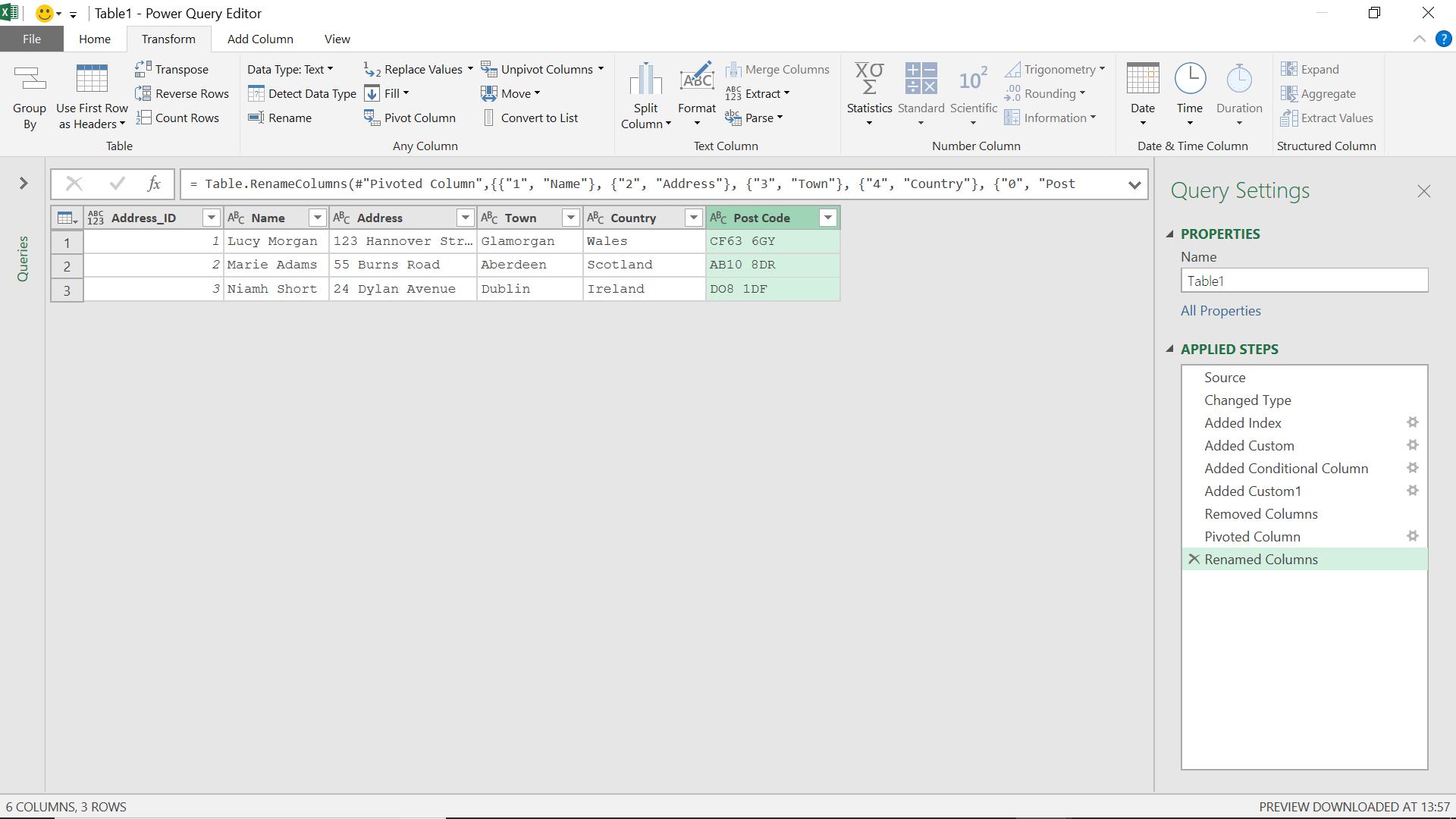
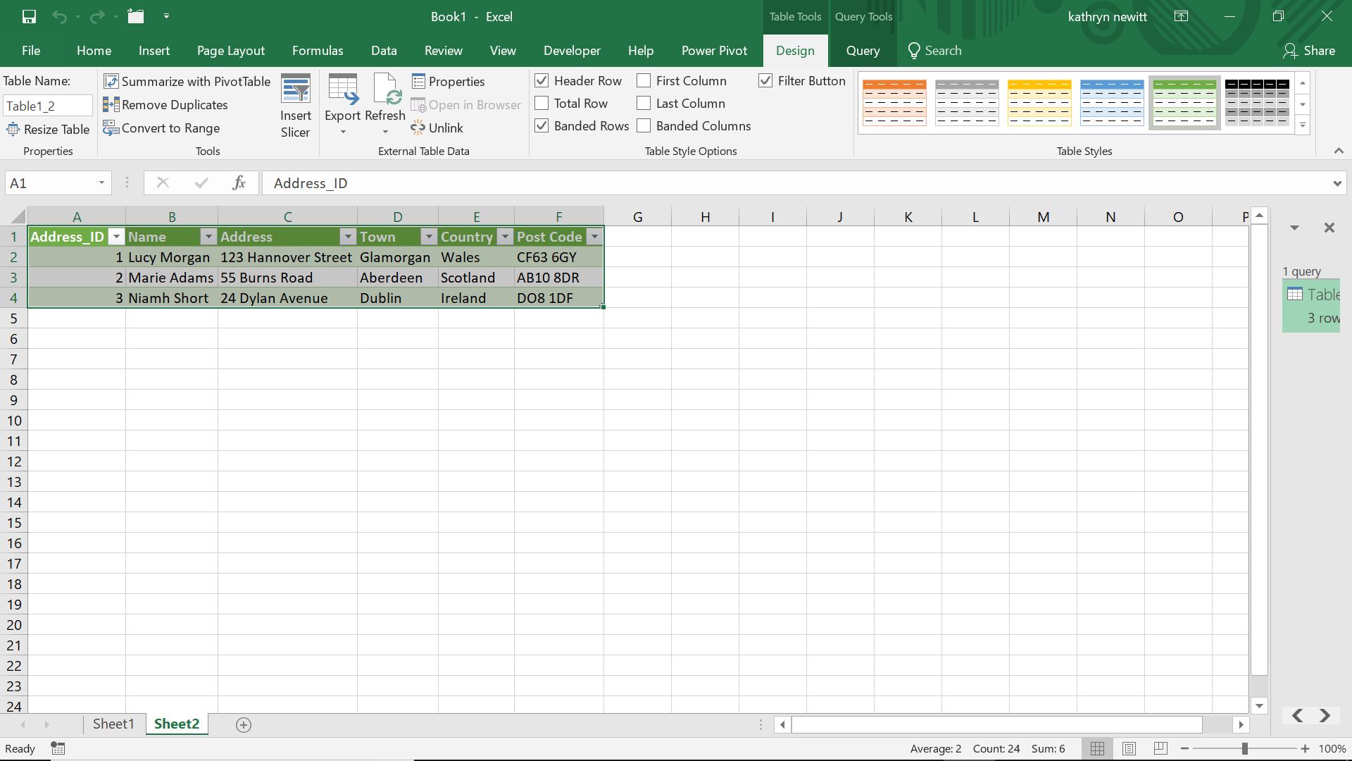
This data is now ready to ‘Close & Load’ to Excel from the ‘File’ tab. If John uses the same Excel worksheet and adds more addresses (or updates any existing ones) then they can be refreshed into the table too.

Want to read more about Power Query? A complete list of all our Power Query blogs can be found here. Come back next time for more ways to use Power Query!