A to Z of Excel Functions: The CUMPRINC Function

Welcome back to our regular A to Z of Excel Functions blog.  Today we look at the CUMPRINC function.

The CUMPRINC function

This function returns the cumulative principal repaid on a loan between a designated start_period and end_period given a constant periodic discount rate.

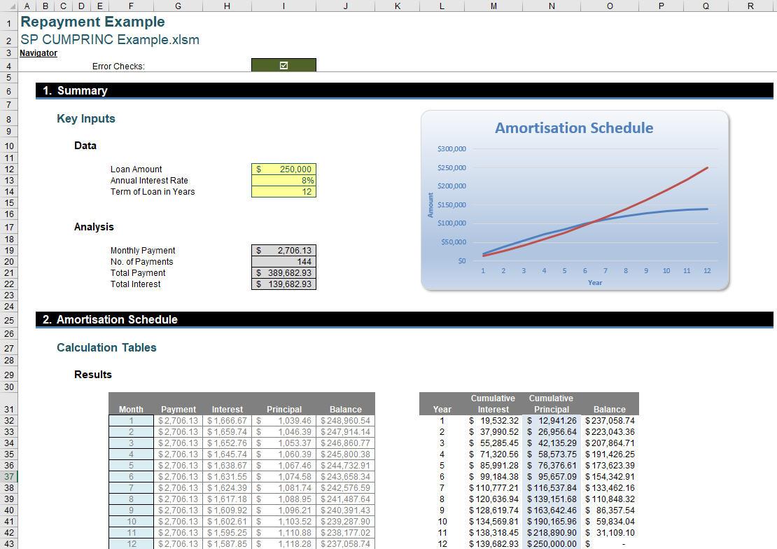
The example illustrated above may be downloaded here.

The CUMPRINC function employs the following syntax to operate:

The CUMPRINC function has the following arguments: 

• rate: this is required and represents the interest rate
• nper: this is also required and represents the total number of payment periods
• pv: this is required and represents the present value of the amount under finance
• start_period: this is required and represents the first period in the calculation.  Payment periods are numbered beginning with 1
• end_period: this is required and represents the last period in the calculation
• type: this is required and represents the timing of the payment.

It should be further noted that:

• make sure that you are consistent about the units you use for specifying rate and nper.  If you make monthly payments on a four-year loan at an annual interest rate of 12 percent, use 12%/12 for rate and 4*12 for nper.  If you make annual payments on the same loan, use 12% for rate and 4 for nper
• if rate ≤ 0, nper ≤ 0, or pv ≤ 0, CUMPRINC returns the #NUM! error value
• if start_period < 1, end_period < 1, or start_period > end_period, CUMPRINC returns the #NUM! error value
• if type is any number other than 0 or 1, CUMPRINC returns the #NUM! error value.

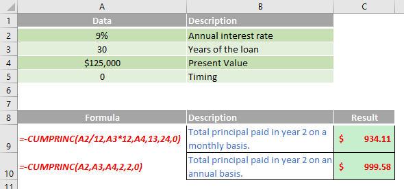
Please see my example below:

Other key points:

• you divide the interest rate by 12 (the number of months in a year) to get a monthly rate, and you multiply the years the money is paid out by 12 to get the number of payments
• in Excel Web App, to view the result in its proper format, select the cell, and then on the ‘Home’ tab and in the ‘Number’ group, click the arrow next to ‘Number Format’ and select ‘General’.

We’ll continue our A to Z of Excel Functions soon.  Keep checking back – there’s a new blog post every business day.

A full page of the function articles can be found here.