A to Z of Excel Functions: The GETPIVOTDATA Function

Welcome back to our regular A to Z of Excel Functions blog. Today we look at the GETPIVOTDATA function.

The GETPIVOTDATA function

To understand the GETPIVOTDATA function, we first need to understand >PivotTables.

Many analysts use Excel to summarise cleaned-up data and convert it into information, with structured (sorted and / or ordered) referencing, so that users may understand their numbers, identify trends and produce various reports.

To understand what I mean, as an example, we may receive data like this:

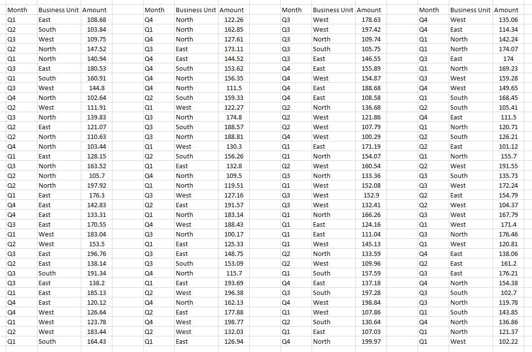
and we may turn it into something more informative, such as this:

Each attribute (known as a field) in a table typically contains a category of data. A crosstab query (similar to the one pictured, above) summarizes the data from one or more of these fields that are separated into groups based on one or more fields. Essentially, a crosstab query summarizes data in more than one dimension to provide insight that may not be immediately forthcoming otherwise. For example, given the source data, how could you possibly notice that Sales for Quarter 4 in the South are very low relative to other quarters and regions?

Excel has many useful tools that will assist, centred around its version of an enhanced crosstab query, known as a PivotTable.

Crosstabs let you quickly compare, contrast and otherwise assess sales activity based on the variables you chose. However, if you sought to deeply analyse the data, you would need to re-design your crosstab query. No such limitation exists with PivotTables.

PivotTables allow you to analyse in two dimensions (row and column), and filter on many parameters. They let you filter, drag, drop, rearrange and drill down on data to create additional reports right on the spot.

Due to their similar appearance, crosstabs and PivotTables are often referred to as the same thing. They are not. While they do have obvious differences, both can be powerful tools for providing deeper insights into your existing data. Here, we will concentrate on PivotTables.

A PivotTable is a semi-dynamic, tabular summary of data. It is one of Excel’s most flexible tools and can provide results that would take some time to reconstruct with sophisticated uses of functions such as SUMIF, SUMPRODUCT, and so on.

Imagine we are a Head Office Analyst reviewing the sales of four divisions: imaginatively called North, South, East, and West. For reasons known only to me, that’s the order I wish to report – neither alphabetically nor reverse alphabetically.

Creating a PivotTable is straightforward. Assuming the dataset is in one block (a ‘contiguous’ range) and has been converted to a Table (Ctrl + T) so that the range may be extended automatically, simply select any cell within the dataset and then click on Insert -> PivotTable (Alt + N + V):

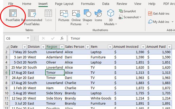
This gives rise to the ‘Create PivotTable’ dialog box:

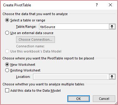
You have the choice of where to place the PivotTable report – either on an existing worksheet (not necessarily the worksheet you are on presently) or else insert a new worksheet.

I have a “rule of thumb” regarding PivotTables.  If you are using them for analysis and the fields may be switched to assess trends / understand the data, then the PivotTable may vary in size considerably.  Therefore, it is best to have the PivotTable on a separate worksheet, with very little else on it, so that it cannot clash with other spreadsheet elements, such as charts, datasets, formulas, and so on.

However, if the PivotTable is more “mature” and is being used to summarize data on an output sheet, then you may put more than one PivotTable on the sheet, as long as you ensure they cannot collide when changing filters.  These sheets tend to be output sheets known as dashboards.  It’s a good idea to place PivotTables at the foot of any such sheet so that if a filter reduces the PivotTable’s footprint significantly, the white space created will not look conspicuous.

Also, remember when selecting where to place a PivotTable, always remember the main PivotTable will be positioned two rows further down.  Do remember if you make a mistake, it’s not the end of the world! You have two options available to you:

1. Move the PivotTable: This is very easy to do. Simply click a cell within the PivotTable. This triggers the context specific ‘PivotTable Tools’ tabs ‘Analyze’ and ‘Design’. On the ‘Analyze’ tab, in the ‘Actions’ grouping, select ‘Move PivotTable’ (Alt + JT + V) and then follow the instructions

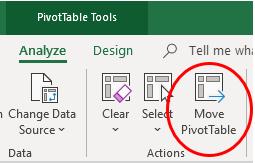
1. Delete the PivotTable: This is even easier to achieve! Simply highlight the entire PivotTable range and select ‘Delete’ on the keyboard.

The PivotTable has four areas where data fields may be placed (a data field is simply any one of the columns of the database, for example, Date, Division, Sales Person, Amount Invoiced, in this illustration):

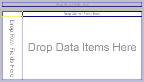
• Page: Values in this field appear as page items in the PivotTable
• Row: Values in this field appear as row items in the PivotTable
• Column: Values in this field appear as column items in the PivotTable
• Data: The field to be summarized – if this data is numerical in nature, SUM (how much) will be the default operation, otherwise COUNT (how many) is used. They are easily changed, if necessary.

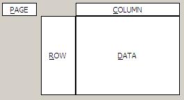
More than one field can be placed in any of these locations – the effect is a hierarchical grouping depending upon the order of placement.

In essence, a PivotTable is a three-dimensional summary of a database. Consider it as a book: each page has a summary table of a selection of the data (for instance, in our example, each page could show the sales of each electrical item for each region and division on a particular date, so Page 1 is 1 1 Jan 20, Page 2 is 2 Jan 20, and so on).

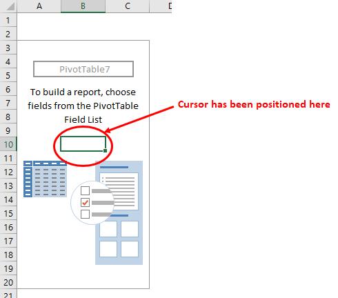
To populate the layout, it is simply a case of dragging and dropping, provided you have the PivotTable Fields pane visible (previously known as the Field List). If it does not appear, right-click anywhere in the PivotTable region and on the shortcut menu select the last item ‘Show Field List’. The PivotTable Fields pane appears when you click inside the PivotTable region:

The PivotTable Fields pane will look similar to this (it can be resized if necessary):

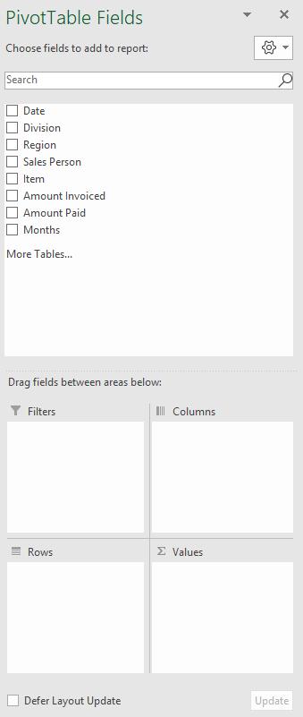
The fields may be dragged into the bottom section, dragging it into one of the four windows below (‘Filter’ is the ‘Page’ equivalent). If I just dragged ‘Region’ in for instance (into ‘Rows’) I would get a sorted, unique list of the regions:

That’s fine, although with the dynamic array functions >SORT and >UNIQUE now available in some versions of Excel (with no need to refresh data as it changes), this may not be as useful a trick as it once was.

As a more comprehensive example, let’s consider I had dragged fields around as follows:

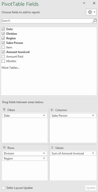
Depending upon your current PivotTable settings, your PivotTable might look something like the following:

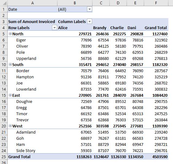
How easy is this? I feel like I am writing under false pretences. The number formatting could be better, the three text fields “Sum of Amount Invoiced”, “Column Labels” and “Row Labels” look a little clunky, but it’s not a bad start.

One great thing about PivotTables is how easy they are to manipulate. Subtotals may be added from the Design tab:

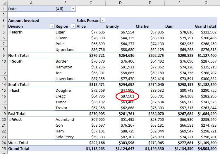
It’s important to realise that your data may move as you modify your PivotTable.  Imagine you wished to link a formula to Brandy’s sales in Eregg (circled).  Here, the cell reference would be D16.  However, after filtering on Date, Division and Sales Person, the PivotTable is restated as

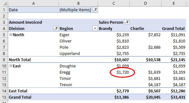
Not only is the value different (due to the Date filter), now the cell reference is C11.  The Excel formula would not move because no rows / columns have been inserted / removed. This is where the function GETPIVOTDATA comes in.

Check File -> Options and then go to Formulas:

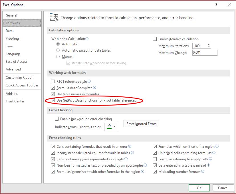
If ‘Use GetPivotData functions for PivotTable references’ is checked, then clicking on the cell containing Brandy’s sales for Eregg would not have provided a typical Excel reference. Instead, it would generate the formula

This should be read as “for the PivotTable with ‘Amount Invoiced’ in its top left-hand corner in cell A3, report back the sales where the Division is East, the Region is Eregg and the Sales Person is Brandy – it’s essentially the PivotTable equivalent of the SUMIFS function.

On a side note, you should also see that our trick from earlier – putting ‘Amount Invoiced ‘ (with a trailing space) has fooled GETPIVOTDATA.

Using GETPIVOTDATA allows you to reference data in the PivotTable as long as it is in the PivotTable!

You can use GETPIVOTDATA to retrieve summary data from a PivotTable, provided the summary data is visible in the report.

Note: You can quickly enter a simple GETPIVOTDATA formula by typing = (the equal sign) in the cell you want to return the value to and then clicking the cell in the PivotTable that contains the data you want to return.

Its syntax is as follows:

It has the following arguments:

• data_field: this is required and represents the name, enclosed in quotation marks, for the data field that contains the data that you want to retrieve
• PivotTable: this is also required.  This is a reference to any cell, range of cells, or named range of cells in a PivotTable.  This information is used to determine which PivotTable contains the data that you want to retrieve
• field1, item1, field2, item2: these pairs of arguments are optional.  If used, you may have from 1 to 126 pairs of field names and item names that describe the data that you want to retrieve.  The pairs may be in any order.  Field names and names for items other than dates and numbers are enclosed in quotation marks.  For OLAP PivotTables, items can contain the source name of the dimension and also the source name of the item.  A field and item pair for an OLAP PivotTable might look like this:
  
  "[Product]","[Product].[All Products].[Foods].[Baked Goods]".

It should further be noted that:

• calculated fields or items and custom calculations are included in GETPIVOTDATA calculations
• if PivotTable is a range that includes two or more PivotTables, data will be retrieved from whichever report was created most recently in the range
• if the field and item arguments describe a single cell, the value of that cell is returned regardless of whether it is a string, number, error, and so on
• if an item contains a date, the value must be expressed as a serial number or populated by using the DATE function so that the value will be retained if the worksheet is opened in a different locale.  For example, an item referring to the date March 5, 1999 could be entered as 36224 or DATE(1999,3,5)
• times may be entered as decimal values or by using the TIME function.
• if PivotTable is not a range in which a PivotTable is found, GETPIVOTDATA returns an #REF! error
• if the arguments do not describe a visible field, or if they include a report filter in which the filtered data is not displayed, GETPIVOTDATA returns the #REF! error value.

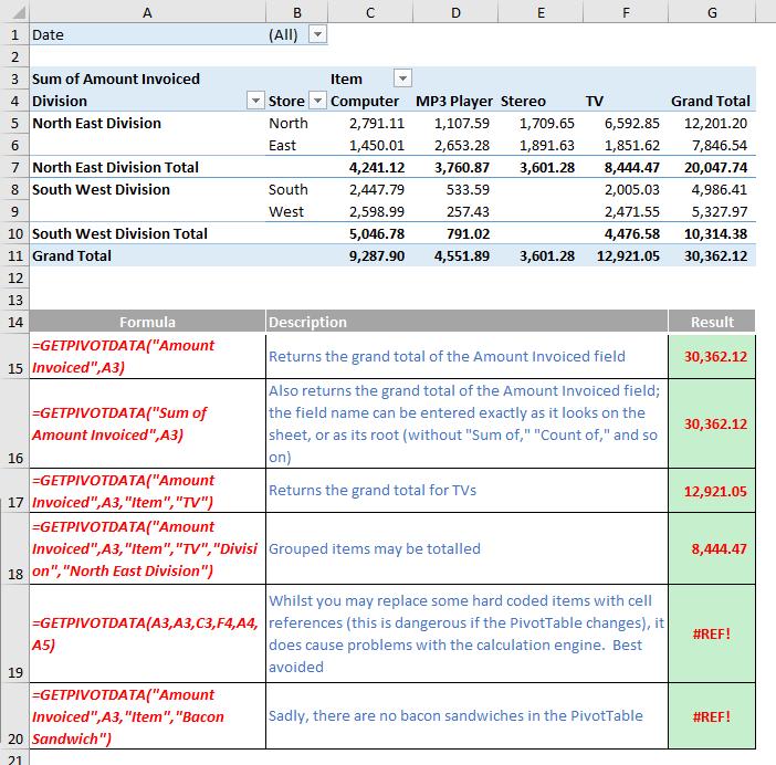
Please see my example below: 

We’ll continue our A to Z of Excel Functions soon. Keep checking back – there’s a new blog post every business day.

A full page of the function articles can be found here.