A to Z of Excel Functions: The LAMBDA Function

Welcome back to our regular A to Z of Excel Functions blog.  Today we look at the LAMBDA function.

The LAMBDA function

Back in November 2020, LET was made Generally Available.  Its sister function, LAMBDA, has been released into the Office 365 Beta world, as at the time of writing.  This function “completes” Excel and provides you with the ability to create your own reusable formulae.

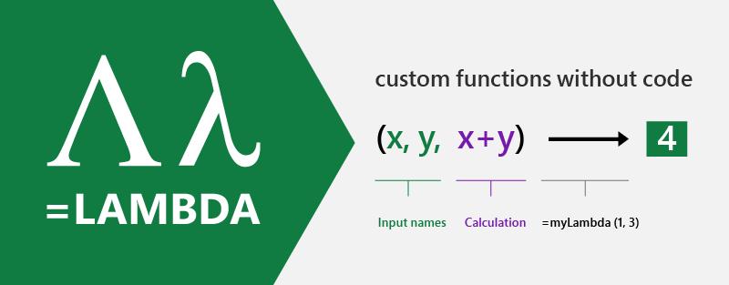
LAMBDA allows you to define a custom function in Excel’s very own formula language.   Moreover, one prescribed function may call another.  If the function calls itself, that’s an example of recursion, which is a way of a function calling itself, called recursion, which is a way… [get on with it – Ed.]

As a reminder, there are three key pieces of =LAMBDA to understand:

1.      LAMBDA function components

2.      Naming a lambda

3.      Calling a lambda function.

1. LAMBDA function components

Let’s take a simple example.  Consider the following formula:

where we have x as the argument, which you may pass in when calling the LAMBDA, and x+1 is the logic / operation to be performed.  For example, if you were to call this lambda function and define x as equal to five (5), then Excel would calculate

Except it wouldn’t.  If you tried this you would get #CALC!  Oops.  That’s because it’s not quite as simple as that.  You need to name your LAMBDA.

2. Naming a lambda

To give your LAMBDA a name so it can be re-used, you have to use the Name Manager (CTRL + F3 / go to the Ribbon and then go to Formulas -> Name Manager):

Once you open the Name Manager you will see the following dialog:

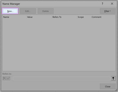
You then click on ‘New’ and fill out the related fields, viz.

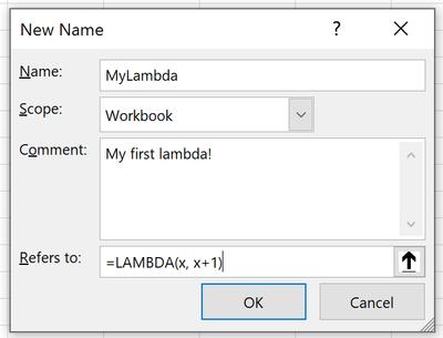
It’s no harder than clicking ‘OK’ at this point.

3. Calling LAMBDA

Now that you have done this, your first new lambda function may be called in just the same way as every other Excel function is cited, e.g.

which would equal six (6) and not #CALC! as before.

You DON’T have to do it this way though if you don’t want to.  You may call a lambda without naming it.  If we hadn’t named this marvellous calculation, and simply authored it in the grid as we had first attempted, we could call it by simply typing:

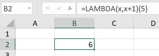
This trick won’t always work though…

LAMBDA’s Aversion to Recursion

To be clear, LAMBDA has no aversion; in fact, it enables it.  But it makes for a great sub-heading.  The “aversion” is that when you use recursion in a LAMBDA,

may not give the expected result.  Instead, it will most likely generate an error, making you think you have written your expression incorrectly.  Let me illustrate with a simple example.  Consider the following:

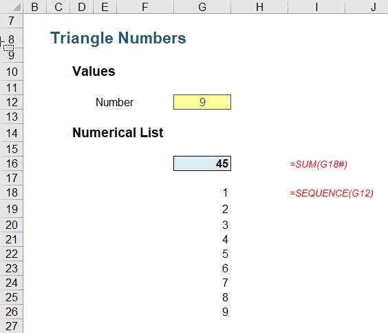
In cell G12, I have typed the number nine (9), which generates the list of numbers one (1) through nine (9) from cell G18 downwards, using the SEQUENCE function, viz.

For those who recognise this is a dynamic array function and that you require Office 365 at this juncture, you are quite right – but I need Office 365 Beta version for the LAMBDA functions, so it’s OK.  I apologise if you don’t have Office 365, but again, you might wish to reconsider which version of Excel and Office you are running, in that instance.

Cell G16 simply sums this list:

Therefore, inputting the numbers one (1) through (9) in cell G12 would generate the results

In cell G16.  These numbers are known as the triangle numbers

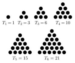
in mathematics, for very obvious reasons.

I want to show you how you can generate this sequence using a LAMBDA.  Now, yes, I know the formula above works and you can even use the algebraic solution

too, but the point is here, I want to show you how to create a recursive LAMBDA function that is simple to follow. 

On the Ribbon, go to the Formulas tab and click on ‘Name Manager’ (as above) (CTRL + F3) and click on the ‘New…’ button.

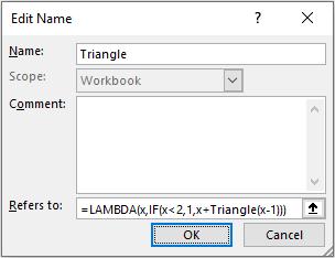
I have named my lambda function Triangle, and the reference (‘Refers to:’) is given by

Here, the lambda function takes a parameter x and defines it as one (1) if it is less than two (2), else it takes the value x and adds the lambda value for x-1 – hence the recursion.  This lambda function has been named Triangle (in the ‘Name:’ box) and is referred to in the formula too.

Therefore, for x equals nine (9):

Drawn out long hand, the recursion is clear.

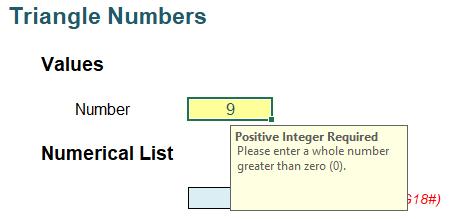
This presupposes that x is an integer, and I have ensured this by incorporating data validation (Data -> Data Validation or ALT + D + L) into my input cell (keep it simple!):

Now that the lambda function Triangle has been defined, the formula in Excel is easy:

I have purposely created a simple recursive formula to demonstrate how such a calculation might work.  In reality, recursive formulae are likely to be much more sophisticated and / or complex. 

Let’s assume that wasn’t the case though, and you wanted to check whether your formula was working.  Not everyone (anyone?) can type a formula and have it work first time, every time.  Many of us would want to try the formula in a cell first:

Oh dear. That didn’t work. Of course it doesn’t. As explained above, it needs the parameter (x) to be defined:

Rats.  This is the problem I alluded to earlier.  My definition of the function refers to itself (i.e. recursion is exhibited).  The name has not yet been defined.

Now watch out here.  Note the function here is Triangle1, not Triangle.  There is a very important distinction.  If I use Triangle, a similar formula will work:

This is very easy to explain.  I have already defined Triangle in the Name Manager!  This is why I am using Triangle1 to avoid this classic gotcha. 

OK, let’s define Triangle1 then.  That will mean wrapping the expression in a LET function.  This allows you to stop writing the same expressions time and time again in a formula, or, as Microsoft puts it, it’s “…names on a formula level”.

This has not worked either, even though Triangle1 has supposedly been cited by LET. The problem is, Triangle1 has not been defined when we are creating the lambda. This where our trick comes in – which also explains the title for this article: it’s all about ME. Let’s add a parameter (ME) to Triangle1, and replace the recursive call to Triangle1 with ME (ensuring you pass in ME as the first parameter):

Believe it or not, we are getting somewhere now.  Even though #NAME? has been replaced with #VALUE!, the formula has evolved.  Assuming you have background error checking enabled (File -> Options -> Formulas -> Enable background error checking), you can click on the error to see the issue:

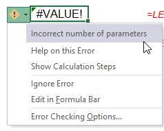
We have an incorrect number of parameters. We have added a parameter to Triangle1 (namely, ME), so the final argument of LET (Triangle1($G$12)) should also have two parameters. We do this by getting Triangle1 to refer to itself, viz.

It works!  We have checked / debugged our LAMBDA in Excel.  We started by calling Triangle1(Triangle1,$G$12), and when we evaluate that lambda, we end up calling Triangle1(Triangle1,$G$12-1), etc. 

This technique has employed the ME parameter: by passing Triangle1 as a parameter to itself, it can then use that parameter to call itself.

Once you've got your head around this, proved for yourself Einstein’s Theory of General Relativity and demonstrated Schwarzschild’s solution to Einstein’s field equations using tensor analysis, you have probably got your lambda working properly!  Now, simply remove all references to ME.  Exclude ME as the first parameter and replace the ME( calls with the defined name you want to use (here, Triangle1).  Therefore, in this instance,

becomes

i.e. we have proved our expression is correct.  We can now add this to the Name Manager.

Taking it Further: Pascal’s Triangle

Sorry to bring back childhood recollections of mathematics, but triangle (or triangular) numbers feature in Pascal’s Triangle:

Starting with a 1 in what is conventionally known as the “zeroth” row (!), each subsequent row’s value is calculated as the sum of the cell directly above it and the cell to the left of the cell above the cell you are in.  Notice the triangle numbers occur in both the third column and the third diagonal from the top.

This is an almost “ultimate” recursion, as you can trace any number on any row back through its constituent elements higher up the Triangle.  Note that this beast is useful in mathematics as this array displays the binomial coefficients of (x + 1)ⁿ.  For example:

• (x + 1)⁰ = 1 – which is the coefficient on the zeroth (0^th) row
• (x + 1)¹ = x + 1 = 1x + 1 – the coefficients 1 and 1 are on row 1 of Pascal’s Triangle
• (x + 1)² = x² + 2x + 1 = 1x² +2x + 1 – the coefficients 1, 2 and 1 are on row 2 of Pascal’s Triangle
• (x + 1)³ = x³ + 3x² + 3x + 1 = 1x³ + 3x² + 3x + 1 – the coefficients 1, 3, 3 and 1 are on row 3 of Pascal’s Triangle, etc.

Now, yes, I know, Excel has a function that calculates these coefficients – and hence any element of Pascal’s Triangle.  If you are often COMBIN the Excel functions to see how many subsets you can make, then COMBIN is for you.  This function returns the number of combinations for a given number of items (i.e. the number of distinct subsets of items where order is unimportant).  You should use COMBIN to determine the total possible number of groups for a given number of items.

The COMBIN function employs the following syntax to operate:

The COMBIN function has the following arguments:

• number: this is required and represents the number of items
• number_chosen: this is also required.  This denotes the number of items in each combination.

However, in the context of Pascal’s Triangle, it may be seen to be

COMBIN(row_number, column_number)

where both row_number and column_number start at zero, rather than one for the reasons demonstrated above.

The technique for calculating this using a recursive lambda function is very similar to the Triangle example (above).  You can define Pascal in the Name Manager (CTRL + F3) as

This may be checked in a cell using the ME technique (as above):

I don’t plan to go through this here, but you may review in the attached Excel file.

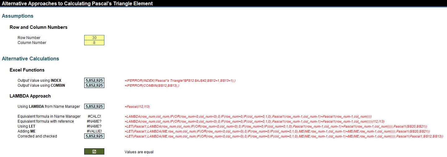
This Pascal lambda function is a more complex example of recursion that highlights an important design consideration.  On my reasonably powerful computer, when I tried to select an element from row 30 of Pascal’s Triangle, Excel took c.55 seconds to calculate, due to all the interim recursive calculations. 

Be careful.  Lambda calculations in Excel are very fast, but if you adopt an excessive recursive approach as I have done here, any powerful PC will be slowed down to a “crawling speed”.  The problem here is that the calculation speed in this instance is proportional to , where n is the row number.

A better lambda might be Pascal_Row, where the time taken is proportional to n²:

This is achieved by calculating on a row, rather than an element, basis.

But even this may be improved upon.  Consider Pascal_Fast:

This is very quick compared to both of the previous alternatives, as the time here is proportional to just n, the row number.  The problem as you may have noticed here, is that as you maximise the iterative approach, the transparency of the calculation – for the average user – tends to become more and more opaque.  PhDs in Computer Science are available upon request.

As a compromise, perhaps

{Pascal_Almost_As_Fast) might work best, which takes approximately twice as long as the above monster (i.e. “almost” instantly).

Care with IFS and SWITCH

Given how calculations may “blow out” quickly when creating iterative functions, it’s best to avoid another classic gotcha.  Let me illustrate with one of the best-known iterative sequences, the Fibonacci sequence:

This sequence is calculated as F_n = F_n-1 + F_n-2.

You might choose to define a lambda function using IFS as follows:

If you are starting to follow lambdas, you should see this appears to make sense (the final argument of IFS, given the criterion is simply TRUE, resorts in advising what to do when x is neither equal to one (1) nor two (2)).  There is a problem though.  This function will run forever, since each parameter in this IFS statement must be evaluated before IFS gets evaluated.  Therefore, when evaluating Fibonacci(1), it will try to evaluate Fibonacci(0) + Fibonacci(-1), and so on.  Not good! 

Therefore, you should use IF instead:

as IF does not evaluate a parameter it does not return.

Be advised, SWITCH exhibits a similar such property, and you should choose to use CHOOSE instead.

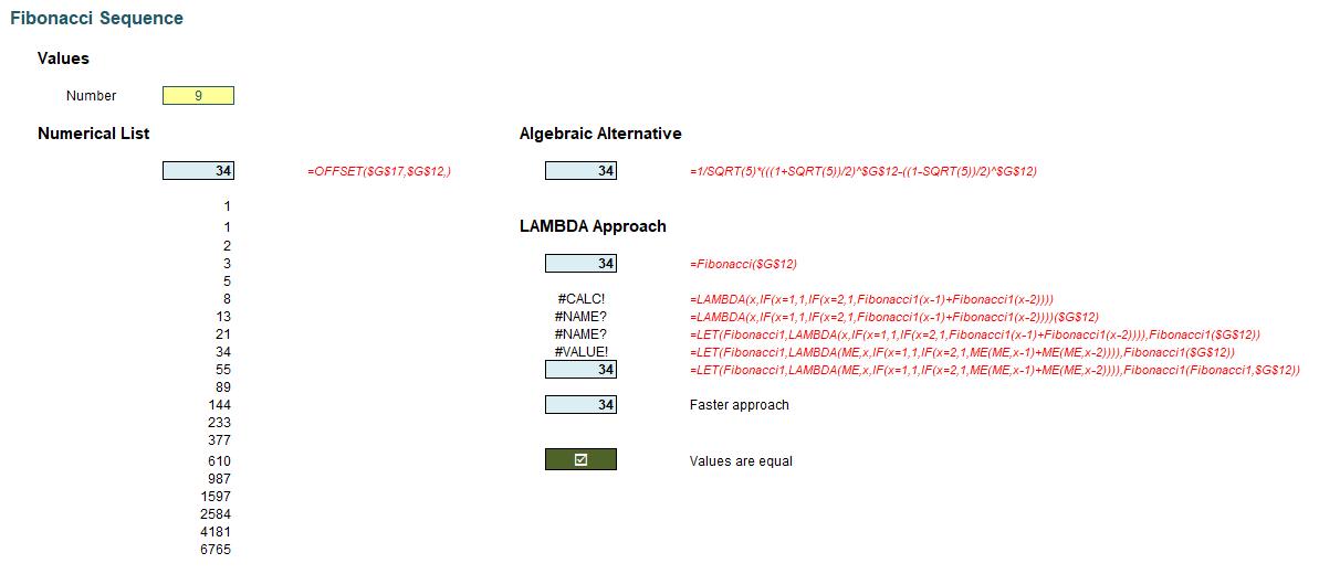
Just to highlight the point earlier about optimisation, the Fibonacci lambda function may be improved upon too – again, at the risk of mathematical / formulaic comprehension:

Now you have something to study the next time you are stranded on a desert island.

Word to the Wise

Playing with new functions is highly addictive and can lead you to using them when they are not needed.  No matter how optimised recursive calculations are, I strongly advise that if you don’t need them, don’t use them.  Formulaic alternatives, such as COMBIN for Pascal’s Triangle are instant and simple, to the naked eye.

Furthermore, do note that the current operand stack limit in Excel is 1,024.  This should be borne in mind together with calculation times, as the current recursion limit is set as 1,024 divided by (number of lambda parameters + 1).

Finally, some common problems faced in financial modelling are not recursive in nature, so try not to confuse the issue unnecessarily.  For example, the most common financial modelling illustration is the calculation of interest on an average cash balance.  This is actually an instance of solving two simultaneous equations.  Applying recursive logic would be inappropriate.