
A to Z of Excel Functions: The RANK Function
24 June 2024
Welcome back to our regular A to Z of Excel Functions blog. Today we look at the RANK function.
The RANK function
The RANK function returns the rank of a number in a list of numbers, i.e. its size relative to other values in a list. In other words, if you were to sort the list, the rank of the number would be its position in the ordered list, be it on an ascending or descending basis.
It should be noted that this function has been replaced with two [2] new functions that may provide improved accuracy and whose names better reflect their usage. Although this function is still available for backward compatibility, you should consider using the new functions from now on, because this function may not be available in future versions of Excel.
For more information about the new functions, see the RANK.AVG and RANK.EQ functions.
The RANK function has the following syntax:
=RANK(number, reference[, order])
It has the following arguments:
- number: this is required and represents the number whose rank you wish to find
- reference: this is also required. This is an array of, or a reference to, a list of numbers. Non-numeric values in reference are ignored
- order: this argument is optional. This is a positional identifier (number)
specifying how to rank number:
- if order is zero [0] or omitted, RANK ranks number as if reference were a list sorted in descending order
- if order is any non-zero value, RANK ranks number as if reference were a list sorted in ascending order.
It should be noted that:
- RANK gives duplicate numbers the same rank. However, the presence of duplicate numbers affects the ranks of subsequent numbers. For example, in a list of integers sorted in ascending order, if the number 10 appears twice and has a rank of 5, then 11 would have a rank of 7 (no number would have a rank of 6)
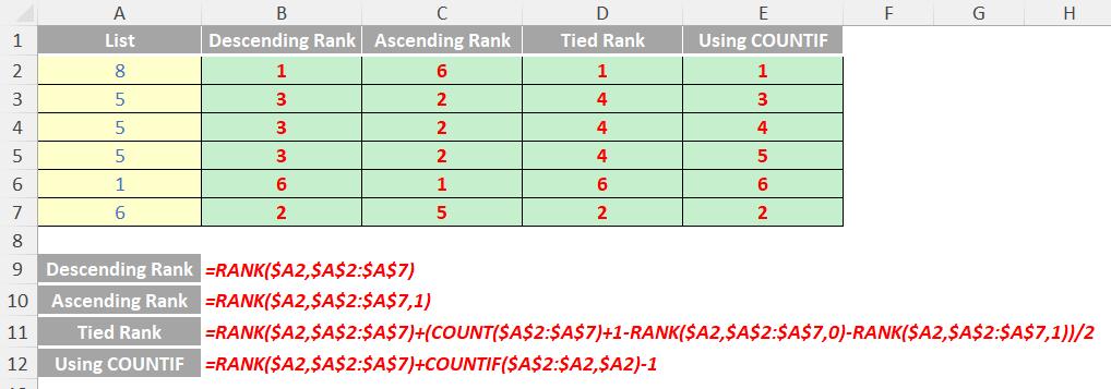
- For some purposes, you might wish to use a definition of rank that takes ties into account. In the previous example, one would want a revised rank of 5.5 for the number 10. This can be done by adding the following correction factor to the value returned by RANK. This correction factor is appropriate both for the case where rank is computed in descending order (order = 0 or omitted) or ascending order (order = non-zero value):
=[COUNT(reference) + 1 – RANK(number, reference, 0) – RANK(number, reference, 1)]/2
- Where “equal ranking” is not required, it is common practice in the modelling community to use COUNTIF to rank items in a list, taking into account the position in the original list as well (see below).
Please see my examples below:
We’ll continue our A to Z of Excel Functions soon. Keep checking back – there’s a new blog post every business day. A full page of the function articles can be found here.