Challenges: Monday Morning Mulling: January 2019 Challenge

On the final Friday of each month, set an Excel for you to puzzle over for the weekend. On the Monday, we publish a solution. If you think there is an alternative answer, feel free to email us. We’ll feel free to ignore you.

Final Friday Fix: January Challenge Recap

This month’s challenge was to convert from US date format (month – day – year) to what is known as the non-US, or more commonly, the European, date format (day – month – year). If you’re in the US, the challenge was the opposite, but the issue and its solution are similar.

The problem arises when you receive date data in a spreadsheet that is not recognised by your regional settings. Therefore, for me, my computer cannot make sense of US date formats such as

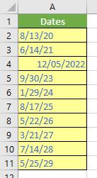
I have left the data in ‘General’ style deliberately so you can see only one entry, cell A4, is recognised as a number (date). The problem is, even that’s wrong as that represents 5 December 2022 not 12 May 2022.

How do I convert it? The simplest answer would be to use Power Query / Get & Transform – but that’s not what I want here.  It may also be done with Excel’s ‘Text to Columns’ feature, but that’s not the solution here either.  I want one formula to do the following:

The Solution

As explained in Friday’s blog, dates are not quite what they seem in Excel. They can cause issues for the unwary, so they are important to understand. For example, August 17, 2008 may be expressed as:

• 8/17/08 (month/day/year, US format)
• 17-8-08 (day – month - year, UK / Europe format, as it’s called by Microsoft, but pretty much anywhere else)
• August 17, 2008
• 17 Aug 2008
• …

Therefore, it does not make sense for Excel to try and force a particular format and many formats are thus supported. Indeed, one thing that is more sophisticated is the fact that whether by default, day comes before month or vice versa is down to your regional settings. This means if I type in

17/8/08

on some computers, this will be recognised as a date, whereas on others it will be seen as a ‘General’ text format because 17 exceeds the number of months in a year. For our American readers, I apologise in advance: my computer is not set to US settings and therefore, the examples here will be displayed as day followed by month followed by year. In the US, the month preceded the day.

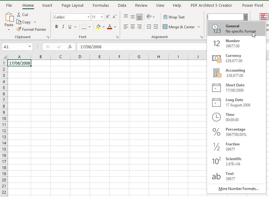
The point is, these are display issues only. As a non-US Excel user, I will type “17/8/08” into cell A1, and then format the cell as ‘General’ (using the drop-down box in the ‘Number’ grouping of the ‘Home’ tab):

This changes cell A1 as follows:

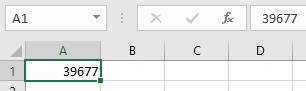
It becomes “39677”, which is known as a serial number (if I were to delete this value, it would make me a serial killer). This serial number is a count from “Day 1” which is defined as 1 January 1900, so Day 2 would be 2 January 1900, Day 3 would be 3 January 1900, and so on. Therefore, according to Excel, 17 August 2008 is Day 39,677.

In essence, we just need Excel to recognise the date as a date – and that was the issue here.

Just to be clear (before everyone writes in!), you can solve this using Power Query / Get & Transform by applying a series of transformations (sometimes it’s just a matter of changing locales, but not always).

For example, if the dates were in an Excel Table (using CTRL + T, called Original_Dates), you could use ‘Get & Transform’ / Power Query by creating a Blank Query,

and pasting the following code into the Advanced Editor:

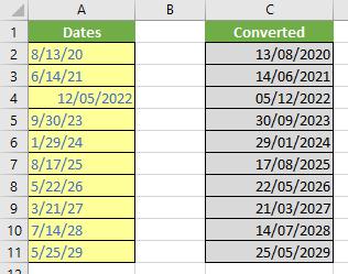
You could also do it in good old Excel by using the ‘Text to Columns’ method as follows. First, I make a copy in cells C2:C11:

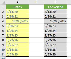
I do this so I may retain the original data (it’s always best to keep a copy in case you make a mistake).

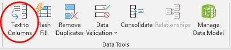
Next, I highlight cells C1:C11 (including the header) and click on ‘Text to Columns’ in the ‘Data Tools’ grouping of the ‘Data’ tab of the ribbon (ALT + A + E):

This generates the ‘Convert Text to Columns Wizard’ dialog box. In ‘Step 1’, choose the ‘Delimited’ option and click ‘Next’.

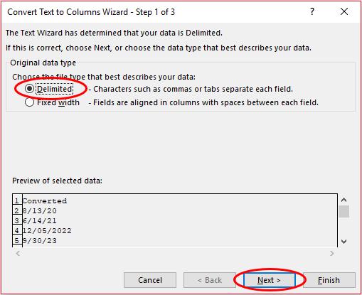
This means the data will be split into columns based upon a specified delimiter. Except we are going to cheat and not do that. In ‘Step 2’, uncheck all delimiters and then click ‘Next’:

Now we come to the step that we actually want. We don’t use the ‘Text to Columns’ feature to split data into separate columns. No, I want Excel to recognize my data as dates.

In this final step, select the ‘Date:’ option in the ‘Column data format’ and choose the date format that matches the data as it currently is – not what you want it to be. You are asking Excel to recognize it. In my case, the data is in Month – Day – Year format (MDY), so this is what I selected. Once you have chosen, click ‘Finish’:

This is arguably the simplest method.

However, both of these methods require data to be refreshed.  The challenge was to construct a formulaic approach.  I must warn you, it’s not pretty, but then, neither am I.  The point is, sometimes brute force and ignorance get the job done.  Here’s my approach in full.

To begin, I convert the date as follows:

The formula

converts cell A2 to a text string in the format day-month-year (which is what you want the data converted to, not the source).  The reason for this is if you used the format code “m/d/yy” instead, cell A4 would have the day and month swapped around incorrectly (as it is already recognised by Excel as a date which is why this value is right-aligned).

The wraparound

is added because for certain regional settings where A2 was originally recognised as a date (like the value in cell A4 here where 5-Dec-22 has been mistaken for 12-May-22), this may cause an error as it is already recognised as a date string.  In this instance, the original value is used instead.

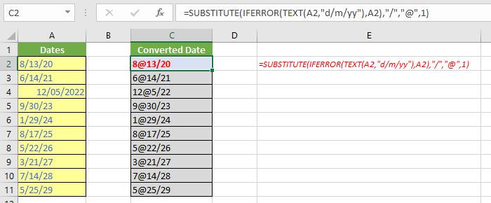
Finally, the formula

uses the SUBSTITUTE function

to replace one or more instances of a given character or text string (old_text) in a text string with a specified character or string (new_text).  The optional instance_number cites the occurrence of old_text you wish to replace.  If this is omitted, all occurrences will be replaced.

Here, I have replaced the first “/” with “@”.  The choice of “@” is arbitrary: I am trying to get the values between the “/” delimiters and having two of these is awkward, so I have replaced the “/” with “@” because I know it’s a character I won’t see in a date text string!

Next, I find the position of the “@” symbol in the text string just created in column C:

is a search function which is case sensitive but does not allow wildcard characters.  It seeks out the first instance of a character or characters (typed in inverted commas) in the within_text text string.  The start_number argument is optional (hence the square brackets in the syntax) so that the first few characters in a text string may be ignored.  If the find_text cannot be located within within_text the error #VALUE! is returned.

Here, the formula

locates the position of “@” in each text string (2 for all but “12/05/2022”).  This is important as we know the first set of numbers (month number) precedes this character and the second set (day number) immediately follows it.

Now we locate “/”:

This is similar to the last formula:

This locates the position of “/” (we aren’t having to hunt for a second one) in each text string.  This is important as we know the numbers before represent the day number and those immediately following represent the year.

We are now in a position to extract the day number:

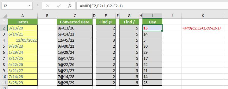
The formula

relies upon the MID function, which is short for “Middle”, which means you can capture parts of a word, starting at any point in a cell.

Its syntax is as follows:

with the following arguments:

• text is as before and refers to the cell / string you wish to convert
• start_number is the starting position (that is, which will be the first character in the text string subset to be extracted).  For example, 2 would mean the second character, 3 the third character and so on
• number_of_characters is the length of the extracted subset text string.

In our formula,

C2 – not A2, which would not work where the value is recognised as a date and has been converted to a serial number – is used as the text.  The start number is the position immediately after the “@” symbol (denoted by E2+1) and the number of characters is the number between the “@” and the “/” symbols, which is given by G2-E2-1 in row 2.

The month number is easier:

This uses the LEFT function:

The text argument refers to the cell you want to convert and [number_of_characters] is the number of characters you want to extract from the cell, counting from the left. The reason the argument is optional (that is, there are square brackets around the second argument in the syntax) is because if it is not specified it is assumed to be one (1).

Here, the formula in cell K2 is given by

where again we refer to C2 as the text (for the same reasons as before).  The number of characters is E2-1, i.e. all of the characters before the “@” symbol. 

The year is just the last two digits of the text string in column C:

This uses the RIGHT function, which works similarly to LEFT, except it starts from the right and counts backwards.  Everything else is the same.  Therefore,

extracts the last two characters of the text string in cell C2.

We just have to put the date together now:

The formula

joins the day, month and year up using “/” delimiters.  However, this is by definition a text string.  Therefore, the actual formula in cell O2,

then converts this to a (serial) number.  Column O has then been formatted as a short date and the Revised Date has finally been created. 

The problem is, we said we wanted one formula.  This means I2, K2 and M2 have to be replaced by their dependent formulae in cell O2, and then these formulae need to keep referencing back too, until all transformations refer back to column A.  When you do this, you get the following wondrous megaformula:

Beautiful.  You can check out the attached Excel file for more details.

The Final Friday Fix will return on Friday 22 February with a new Excel Challenge.  In the meantime, please look out for the Daily Excel Tip on our home page and watch out for a new blog every other business workday.