Challenges: Monday Morning Mulling: November 2018 Challenge

Last week, we posed a challenging question – given a large table of data, how can we create a set of data validated cells that would automatically update when you select a particular item in the previous cell?

We gave you several restrictions:

• The solution needed to be scalable. Creating named ranges for each new type of make and model of vehicle was not acceptable, as it requires additional work should the data update and change.
• The solution needed to deal with the awkward situation that different models of cars would all be made in the same year, so you couldn’t just create a ‘2018’ named range.

The solution we have isn’t trivial, by any means. It comes in two parts – transforming the dataset into a more useable format for our purposes, and then building the data validation framework.

Transforming the dataset

The first task is to convert the dataset into something more useable. Essentially, we need to establish a relationship between Make and Model, in a logical way. This is actually surprisingly difficult. It’s easy to use a Group By command in Power Query to get to here:

… but it’s quite difficult to establish it in two rows or two columns like the following:

To do this, we further grouped the previous values into Tables, as follows:

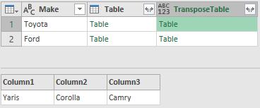
Then, we created a custom function that would transpose the table and keeping only the models in the result:

Removing the Table column and expanding the TransposeTable column then gives us our final result.

We then just needed to repeat these steps to create relationship tables between Model and Year, and Model, Year and Variant.

Building the data validation framework

Once those tables are in place, we essentially need a tool that would look up the first value (the Make of a car) and use that to find the corresponding models associated with that make. To do this, we created a simple table to find the right values.

To populate this table, we’re using a simple INDEX(MATCH) to look for the Make in the first column of our Make / Model table, then specifying the column we want to pull in based on the index number in the list.  So the formula looks like this:

… where G22 is the number in the left hand column of the picture.

So this tells us what models are linked to an input make.  To turn this into a data validation list without the unused cells, we can create a Named Range called “List_Models”, that refers to the cells:

H22 is the first item (currently Fiesta).  Starting from there, it picks up a range that is X rows tall, being the number of non-zero values in the list (in this case, only two).  We can then go into our input cell and set our data validation to point to the List_Models named range:

All we need to do is repeat this process for each different parameter that we have! One Power Query output and one of these validation tables for every field after the first one. Then, we have one named range for each of those fields.

Summary

This is a bit more convoluted than what you’ll find on Google, but it’s a far more flexible and scalable way to build multiple data validation lists that require very little (if any) additional rework once the file has been set up.

How did you go this month? Let us know at contact@sumproduct.com if you like this solution, or if you found another way of getting to the answer. See you next month!