Charts and Dashboards: Interactive Charts – Part 2: Form Controls (Continued)

Welcome back to this week’s Charts and Dashboards blog series. This week, let’s continue our consideration of Form Controls. Here, we look at how to create a Drop-down List using them.

To recap, with Form Controls, we can add a data selection option to charts, for example, through a Check box or a Drop-down List. In the previous blog, we discussed how to create Check Boxes using Form Controls. Now, let’s see how we may create a Drop-down List.

First, in the chart data area, we will add a column, e.g. ‘Sales by group’, with which we will later build our chart. We will also add a list of Groups, with a blank cell at the top (highlighted in green in the image below). Later, we will add a cell link to this.

We navigate to the Developer tab on the Ribbon. We choose Insert -> Form Controls and click the Combo Box (the second left icon on the top row):

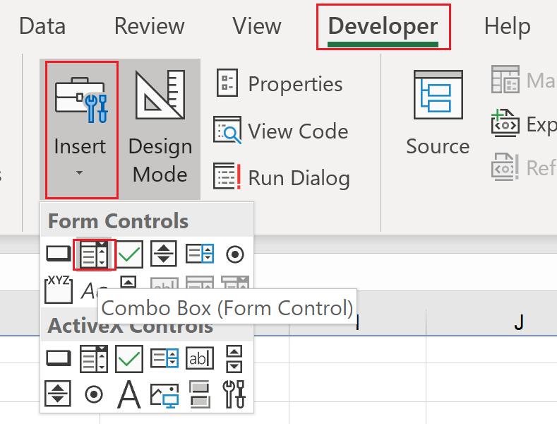
We need to make sure we choose the Combo Box from the ‘Form Controls’ group, not the ‘ActiveX Controls’ group – which is for VBA. If you inadvertently choose the wrong version, you will notice that there is no Control tab in the ‘Format Control’ dialog:

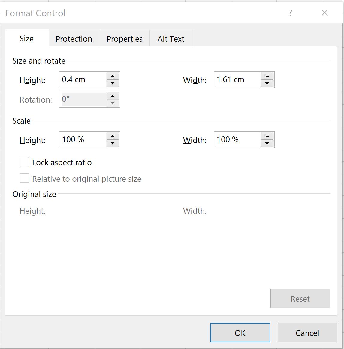
Having selected the Form variant, by holding the ALT key and click on a cell in the worksheet, a box with an arrow icon will appear that may be snapped to grid:

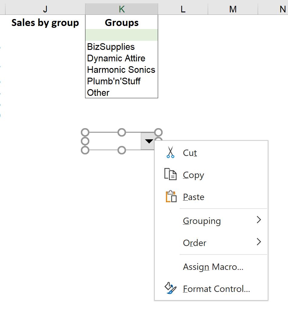
Next, right-click on the icon on the work sheet and click ‘Format Control…’. In the Control tab, to define the ‘Input range’, we will select the list of groups in cell K12:K16, and refer the ‘Cell link’ to the blank green cell, which is cell K11.

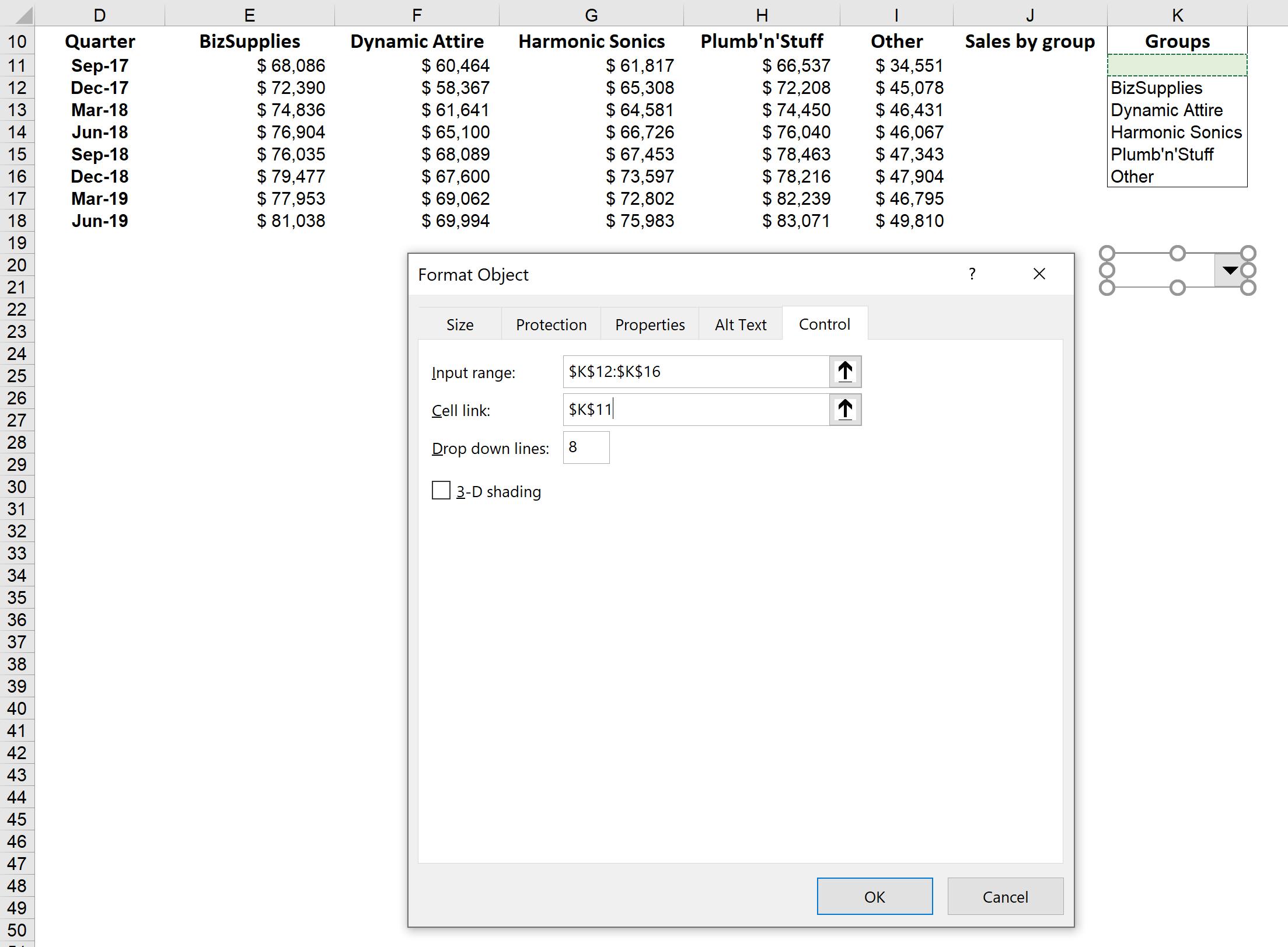
Then, we will resize the arrow box (if necessary). As we choose one item from the list, note that the cell link will reflect its index number (i.e. position in the list):

Now, we need to match the sales figures corresponding to the group that we have chosen from the drop-down menu.  This can be done easily using the INDEX function.  The ‘Sales by group’ cell will be the index result from the corresponding range chosen; the array in this example has only one row, so only one reference is required, whether the range were to consist of one row or one column.  Here, if we choose Biz Supplies from the list, the cell link shows number one (1) – as this is the order of Biz Supplies item in the list, this will also be the column number to index.

The formula in cell J11 is:

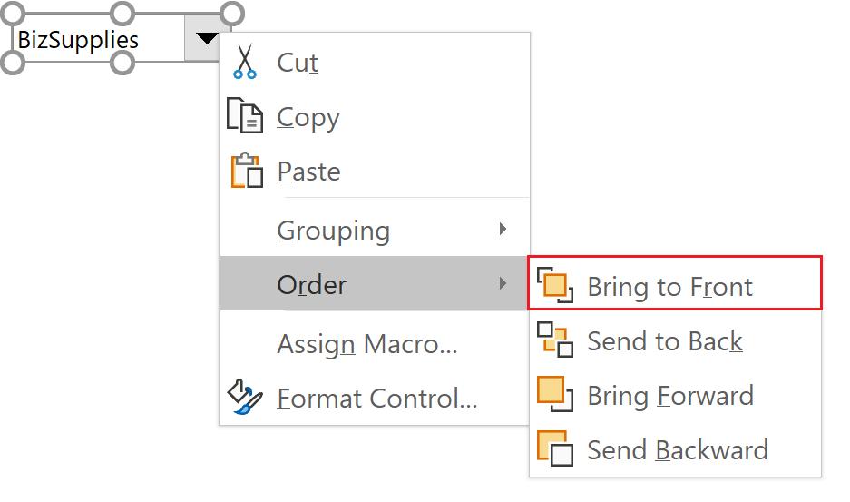
Then we can build a chart on the ‘Sales by group’ column based on Quarters. We may also need to bring the drop-down box to front to insert to the chart. To insert the Drop-down List, just drag the icon to the chart:

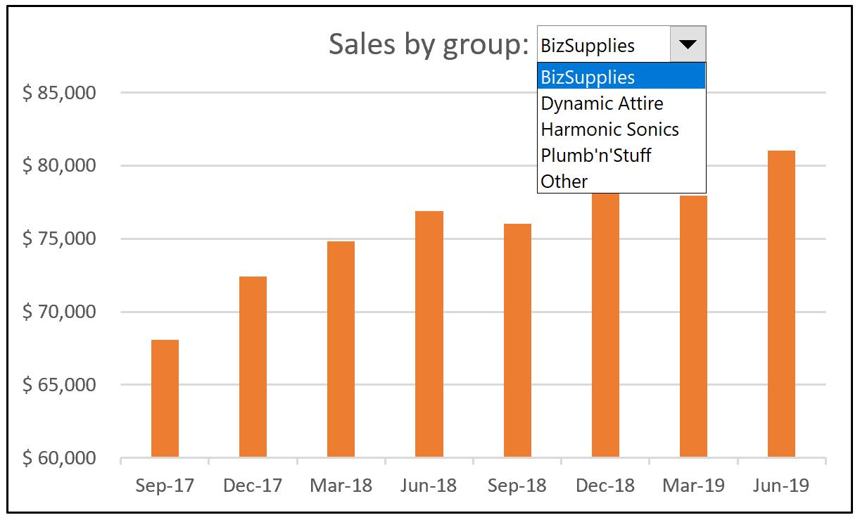
This chart is now interacted accordingly to our group selection using the Drop-down List.

That’s it for this week, check back next week for more Charts and Dashboards tips.