Charts and Dashboards: Dynamic Arrays in Charts
4 November 2022
Welcome back to our Charts and Dashboards blog series. This week, we’re going to look at how charts interact with dynamic arrays.
Historically, creating a chart that updates dynamically to display a different number of data points was a complicated process requiring the use of an Excel Table, Named Ranges or the OFFSET and / or INDEX formula(e). This is no longer the case.

Let’s work through this example to see what’s going on here.

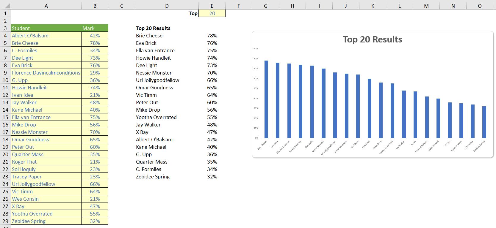
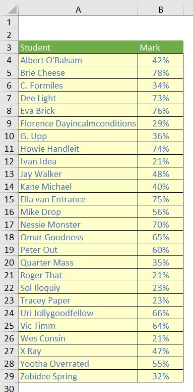
Cells A4:B29 contain our data for this example, and are intentionally not placed within an Excel Table.

Cell E1 contains an input number for use in the formulae in cells D3 and D4. D3 contains the formula
="Top "&E1&" Results"
to provide us with a dynamic title for our graph that will update in line with the figure in E1. The following dynamic array formula is in cell D4:
=INDEX(SORT(A4:B29,2,-1,FALSE),SEQUENCE(E1),{1,2})
This will summarise the top X students (in accordance with the input in cell E1).

Finally, we have inserted a chart in the usual way, linking it to the dynamic range (cells D4:E23 in our example). We have linked the Chart Title to cell D3 so that this will also update dynamically.
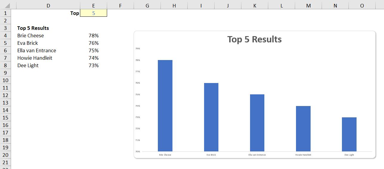
It’s that easy! Now changing the figure in cell E1 to five [5] (for example) will update both our dynamic range of data and the chart, viz.

That’s it for this week. Come back next week for more Charts and Dashboards tips.

