Monday Morning Mulling: December 2020 Challenge

On the final Friday of each month, we set an Excel / Power Pivot / Power Query / Power BI problem for you to puzzle over for the weekend.  On the Monday, we publish a solution.  If you think there is an alternative answer, feel free to email us.  We’ll feel free to ignore you.

The challenge on Christmas day was to spill a range of cells – “Happy New Year” multiple times using Excel formulae.

The Challenge

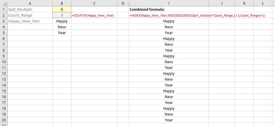
When we say “spill”, we are referring to an Excel formula that returns a range of cells according to user’s needs.  Data often needs to be organised and arranged in different ways.  Now the challenge for this is to spill “Happy”, “New” and “Year” six times each as shown in the example below: 

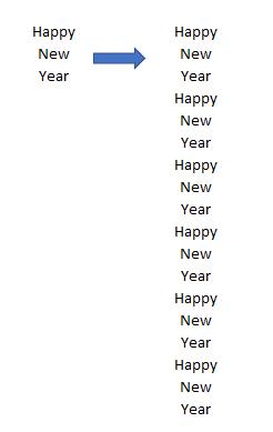
This challenge is designed to get you to think outside the box and beyond your basic functions of copy and paste.

Suggested Solution

We are sure you have solved this Friday’s problem (it’s Christmas after all!). In case you want to check your solution, keep reading through.

First and foremost, create a Dynamic Range Name as follows.

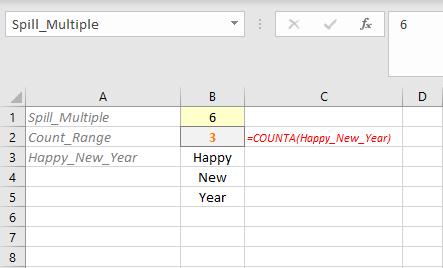
Let’s enter a spill multiple (6) in cell B1 and a count range (i.e. how many items, so “Happy”, “New” and “Year” are three items) for cell B2.  Note you have to use the COUNTA function, not COUNT, as the former counts non-blank cells, whereas the latter only counts numbers.  We use cell B1 to input the number of times that the Happy_New_Year range needs to be spilled and name it as Spill_Multiple, and cell B2 to calculate the range count, named as Count_Range. 

For the stipulated in cell B3, we use the OFFSET function.  To create this, navigate to the Formulas tab on the Ribbon and choose ‘Define Name’, where we will define the name as follows:

Now, let’s go through how to spill the range.

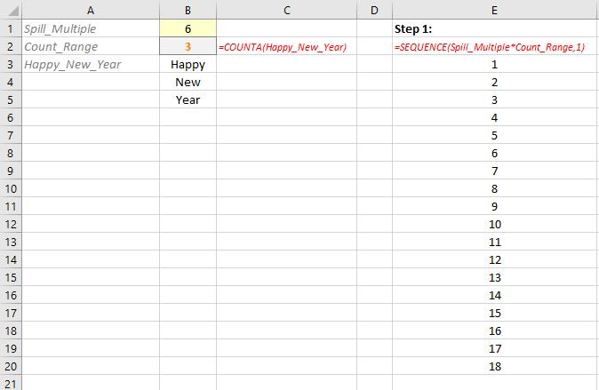
First, we use the >SEQUENCE function to calculate the number of rows this will need to spill over (e.g. if it is six times for an expression three lines deep, we will need a total of 3 x 6 = 18 lines.  SEQUENCE will set up a counter from 1 to 18 for us down 18 rows).

The formula in cell E3 is given by

Excel will forgive you if you choose not to employ the second argument (1).  This is the assumed default value in any case.

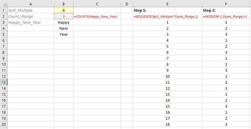
Next, find the index order of the sequencing of Happy_New_Year (i.e. first word, second word, third word, then repeat a further five times).  Here, we may use the MOD function.  This function is used to return the remainder after the number (the first argument) is divided by the divisor (the second argument).  The formula in cell F3 is:

Once we have the indexing, the next step is to simply to “index” the numbers to the text – Happy_New_Year.  The >INDEX function is used to return a value or the reference to the value from within a table or range (list).  In this case, it will match the index order in column F with the Happy_New_Year range that needs to be spilled.  The formula in cell G3 is:

Even better, if you are an Excel expert you may have combined all three steps into one as shown below.  The formula in cell I4 is:

We’re good to go! Happy New Year 2021!

The Final Friday Fix will return on Friday 29 January 2021 with a new Excel Challenge. In the meantime, have a great new year and please look out for the Daily Excel Tip on our home page and watch out for a new blog every business workday.