Monday Morning Mulling: December 2023 Challenge
1 January 2024
Happy New Year! On the final Friday of each month, we set an Excel / Power Pivot / Power Query / Power BI problem for you to puzzle over for the weekend. On the following Monday, we publish a solution. If you think there is an alternative answer, feel free to email us. We’ll feel free to ignore you, but we do appreciate your enthusiasm!
The Challenge
Last Friday, we presented a word puzzle challenge: imagine that you’re presented with an intriguing linguistic challenge: to craft a list of words from a specified set of letters. Manually filtering every single keyword and copying / pasting them to a new location can be a tedious and time-consuming process. We provided you with two Excel Tables: List_of_Letters and List_of_Words.
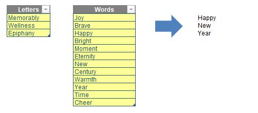
Your objective was to develop one [1] dynamic Excel formula which would look up words from List_of_Words that may be formed from letters of a single word in List_of_Letters, as shown in the picture below:

For example, if the word ‘Epiphany‘ were included in the List_of_Letters and the word ‘Happy’ appeared in the List_of_Words, the formula would check if all letters of the word ‘Happy’ were present in at least one word from the List_of_Letters. Since the letters ‘H’, ‘A’, ‘P’, and ‘Y’ are all found in the word ‘Epiphany’, the word ‘Happy’ will be included in the filtered list. You may download the question file here.
As always, there were some requirements:
- no Power Query / Get & Transform or VBA was allowed
- the formula(e) should be dynamic so that they should update when a new entry was added
- the solution should be case-insensitive, e.g. ‘E’ and ‘e’ should be treated similarly.
Suggested Solution
You can find our Excel file here, which shows our suggested solution. The steps are detailed below.
The Formula
Here’s one way to approach this problem using Excel’s dynamic array functions and text functions.The solution provided is based upon the idea of checking whether all characters in each word from the List_of_Words exists in any one of the words from the List_of_Letters.
=FILTER(List_of_Words[Words],
BYROW(List_of_Words[Words],
LAMBDA(input,OR(BYROW(List_of_Letters[Letters],
LAMBDA(r, AND(ISNUMBER(SEARCH(MID(input,SEQUENCE(LEN(input)),1),r)))))))))
Don’t worry if you do not understand the formula above. Let's go through it step-by-step:
Creating a Sequence of Numbers
To begin, we need to extract all characters from each word in List_of_Words. This may be constructed using a combination of the MID and SEQUENCE functions:
=SEQUENCE(LEN(input))
The formula generates a sequence of numbers from one [1] to the length of the input word, serving as the start number for the MID function to extract each character. For instance, if the input word is ‘Happy’, this step would generate the sequence [1, 2, 3, 4, 5], if the input word is ‘Bright’ it generates the sequence [1, 2, 3, 4, 5, 6].
In the formula above, ‘input’ refers to the current word being processed from the List_of_Words. As the formula iterates through the List_of_Words, it assigns each word to the variable ‘input’ and uses it to evaluate the subsequent expressions.

Note that we will break down a complex formula into manageable steps. This is why in the highlighted cells in red we will refer to specific cells. This approach facilitates a clearer understanding of the calculation complexity.
Extracting Letters
The MID function then extracts a single character from the current word at each position in the generated sequence. The one [1] at the end indicates that only a single character should be extracted.
=MID(input,SEQUENCE(LEN(input)),1)

Searching for the Extracted Letter
The SEARCH function will return a position number if the keywords are found within the text string. Otherwise, it will return #VALUE! error. Then, the ISNUMBER function checks whether the output of the SEARCH function is a number or not and will return TRUE or FALSE accordingly.
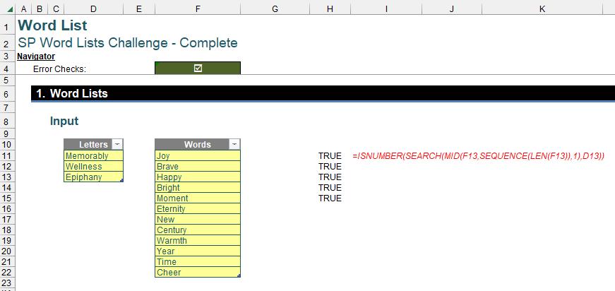
=ISNUMBER(SEARCH(MID(input,SEQUENCE(LEN(input)),1),r))
Here, ‘r’ represents the current word being compared from the List_of_Letters. The SEARCH function checks if the extracted character from the input word is present in the current word from the List_of_Letters.
Using the input word ‘Happy’, the function above compares with the word ‘Epiphany’ from the List_of_Letters, and you can see the result below:

Validating Letter Extraction Against List_of_Words
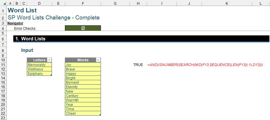
=AND(ISNUMBER(SEARCH(MID(input,SEQUENCE(LEN(input)),1),r))))
Here, the AND function ensures all extracted characters from the current word are found in at least one word from the List_of_Letters. If all characters are found, the result will be TRUE. Otherwise, it will be FALSE. This is a “safe” use of AND, as this does not always play nicely with multiple vectors or arrays.

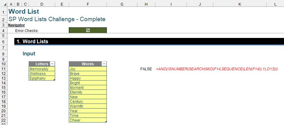
By utilising the input word 'Bright', the function mentioned above is employed to compare it with the word 'Epiphany' from the List_of_Letters. Since not all the letters are present, the returned result is FALSE.

Filtering Condition for Results
This part of the formula applies a function to each row (word) in the List_of_Words. The function is defined as follows:
=BYROW(List_of_Words[Words], LAMBDA(input, OR(BYROW(List_of_Letters[Letters], LAMBDA(r, AND(ISNUMBER(SEARCH(MID(input,SEQUENCE(LEN(input)),1),r))))))))
Let’s break down the function further. This inner BYROW function checks if the current character of ‘input’ in the List_of_Words is present in the current word ‘r’ in the List_of_Letters as mentioned above. It uses a nested BYROW to iterate through each word ‘r’ in List_of_Letters.
In addition, the OR function checks if any iteration of the inner BYROW returned TRUE (meaning all characters were found in any word from List_of_Letters).
This formula essentially acts as a filter condition that returns TRUE or FALSE for FILTER function.

The Final Formula
Finally, after explaining how the functions nested in the formula work. The final formula is as follows:
=FILTER(List_of_Words[Words], BYROW(List_of_Words[Words],LAMBDA(input,OR(BYROW(List_of_Letters[Letters],LAMBDA(r, AND(ISNUMBER(SEARCH(MID(input,SEQUENCE(LEN(input)),1),r)))))))))
The FILTER function in the formula plays a crucial role in filtering the list of words based on a specific condition. The first argument passed to FILTER is List_of_Words, which represents the original list of words you want to filter. The second argument is an expression that utilises nested BYROW and LAMBDA functions to check if each word in the original list meets the filtering criteria and determines which words to keep. This results in a new list containing only words satisfying the condition above, and in our example, the output has a seasonal message from SumProduct for you:
"Happy New Year"

Word to the Wise
We appreciate there are many, many ways this could have been achieved. If you have come up with an alternative, radically different approach, congratulations – that’s half the fun of Excel!
The Final Friday Fix will return on Friday 26 January 2024 with a new Excel challenge. In the meantime, keep honing your Excel skills with our Daily Excel Tip on our home page, and look out for more informative blogs every business working day.

