Monday Morning Mulling: February 2023 Challenge

On the final Friday of each month, we set an Excel / Power Pivot / Power Query / Power BI problem for you to puzzle over for the weekend.  On the Monday, we publish a solution.  If you think there is an alternative answer, feel free to email us.  We’ll feel free to ignore you.

The Challenge

Have you ever thought of putting an interactive picture within Excel that changes with just a simple press of the F9 key on your keyboard?  This month, we challenged you to do that.  You could download the question file here.

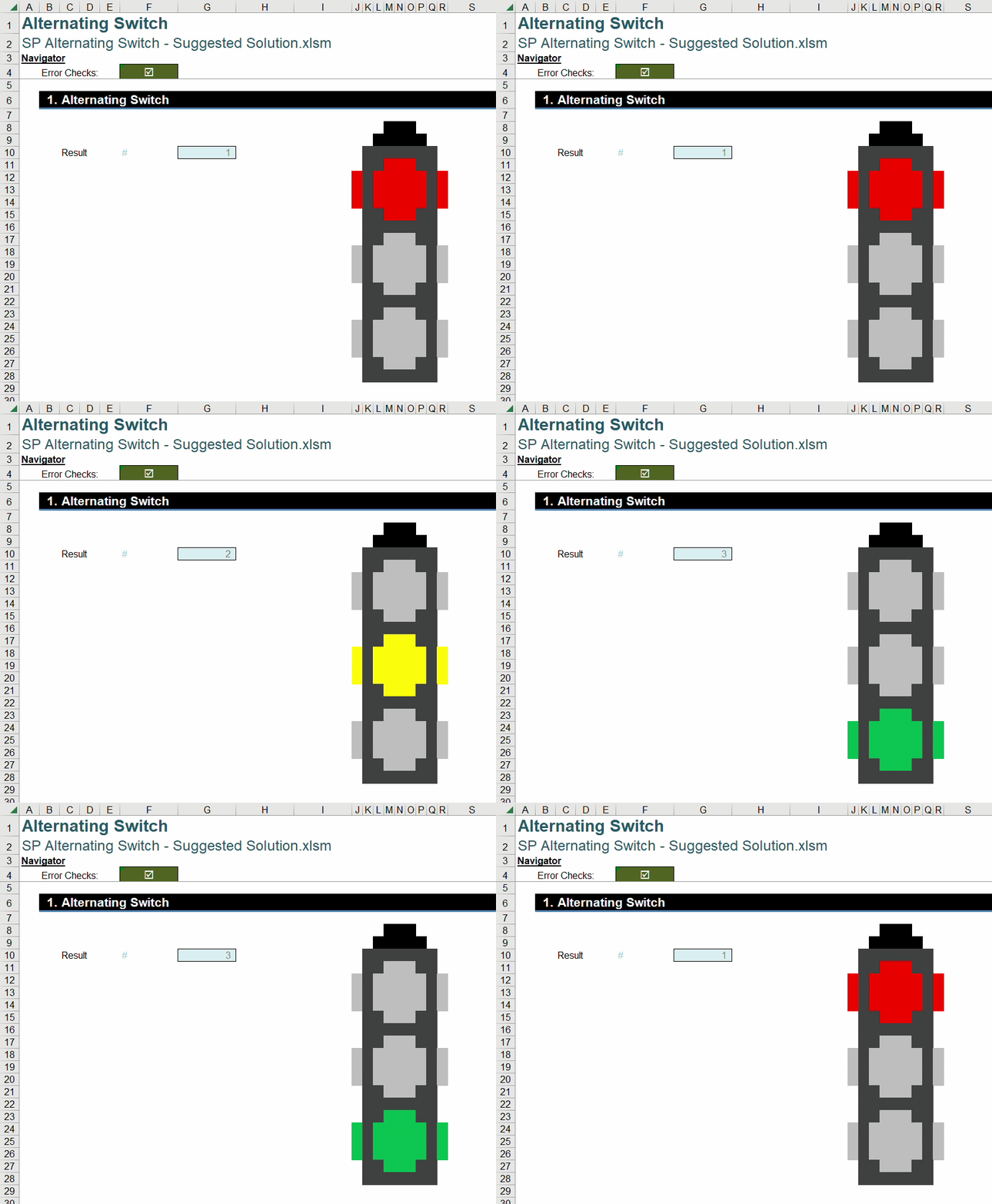
This month’s challenge was to build a cell that could alternate between at least three [3] different values each time Excel recalculates (by pressing F9) and use these values in conditional formatting to make the traffic light flash as shown below:

As always, there were some requirements:

• no Power Query / Get & Transform, VBA or circular reference(s) was allowed
• the traffic light should always alternate in a loop from red to yellow to green and then red again, etc.

Suggested Solution

You can find our Excel file here, which shows our suggested solution. 

To begin with, we have an input cell to enter the number of values in one alternating loop.  In this case, we will enter three [3] as we want the traffic light to switch between three [3] colours which are red, yellow (amber) and green: 

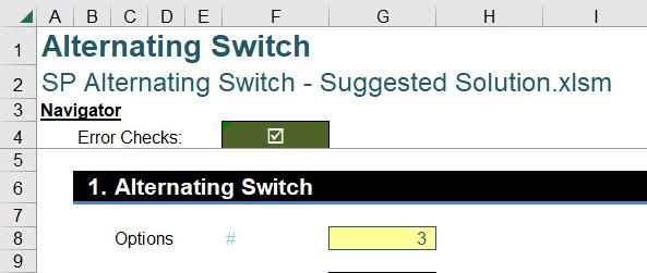
We have named this assumption cell Number_in_Loop.  Then, we have another cell for the outputs with the name Result:

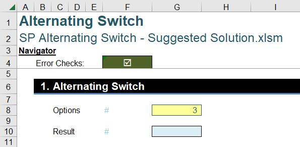
We will leave the Result cell empty for now.  Next, we will prepare a Data Table.  In the column input of the Data Table (i.e.cell H13), we let this cell equal Result:

 In the row input of the Data Table (i.e. cell G14), we enter the following formula: 

This formula calculates the next number in a loop when the Result is changed.  The final step is to create the Data Table.  We will select the whole range G13:H14, go to the Data tab, select What-If Analysis and then Data Table (or ALT + D + T):

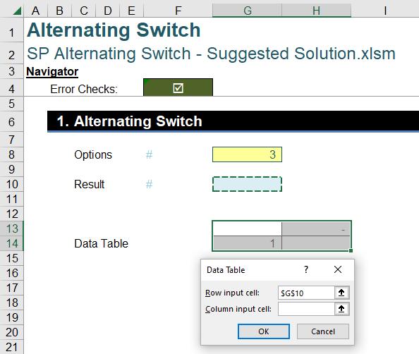
In the ‘Row input cell’ box, we select the Result cell, cell G10.

The finishing touch for this alternating switch is that in the Result cell, we set this equal to the output of the Data Table which is located in cell H14:

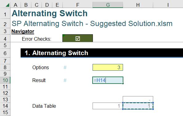
After clicking OK, the row input of the data within the Data Table will calculate once and then stop.  Then, the Data Table’s output will go to the Result cell which makes the ‘Row input’ and ‘Column input’ of the Data Table change.  However, the Data Table will not update until we press the F9 key to force Excel to recalculate.  This way we can avoid the circular reference within the model:

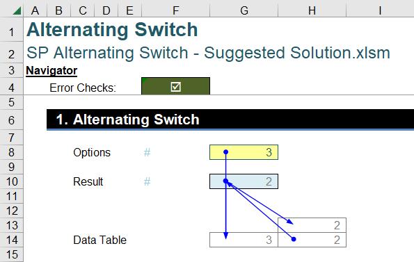
At this point, we are partially done with the challenge.  As we can see that every time the F9 key on the keyboard is pressed the number in Result will increase by one [1] and loop back to one [1] after reaching three [3].

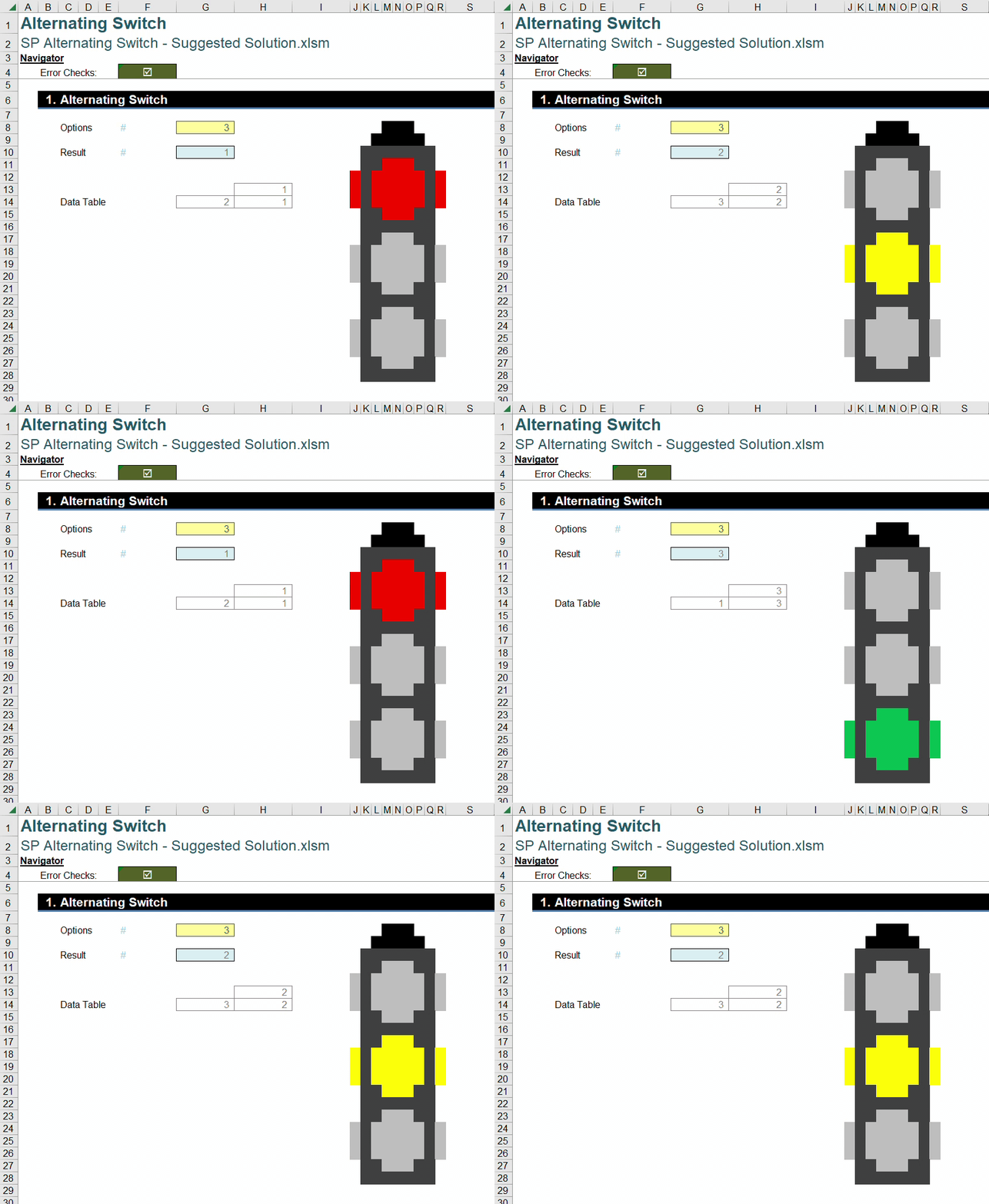
The final step we need to implement here is to use conditional formatting to add the fading colour to the traffic light.  To begin, select the red light region and go to Home -> Styles -> Conditional Formatting ->New Rule (or ALT + O + D).  We select the last ‘Rule Type’ which is ‘Use a formula to determine which cells to format’ and in the formula box below we enter the following formula and apply a light background colour format:

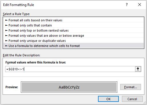
If the Result is different from one [1], the red light will have a grey colour.  We can repeat the same process for the yellow and green lights, using the numbers two [2] and three [3] respectively.  Finally, we have our interactive traffic light, shown below:

Word to the Wise

We appreciate there are many, many ways this could have been achieved.  If you have come up with an alternative, radically different approach, congratulations – that’s half the fun of Excel!

The Final Friday Fix will return on Friday 24 March 2023 with a new Excel Challenge.  In the meantime, please look out for the Daily Excel Tip on our home page and watch out for a new blog every business working day.