Monday Morning Mulling: July 2024 Challenge

On the final Friday of each month, we set an Excel problem (or something similar!) for you to puzzle over for the weekend.  On the Monday, we publish one suggested solution.  No-one is stating this is the best approach, it’s just the one we selected.  If you don’t like it, lump it – or contact us with your preferred solution.

The Challenge

This month’s challenge was to dynamically substitute text in a dataset.  Specifically, you needed to replace certain keywords in a text string with their corresponding substitutes from another list.

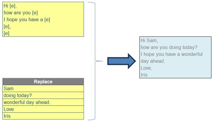
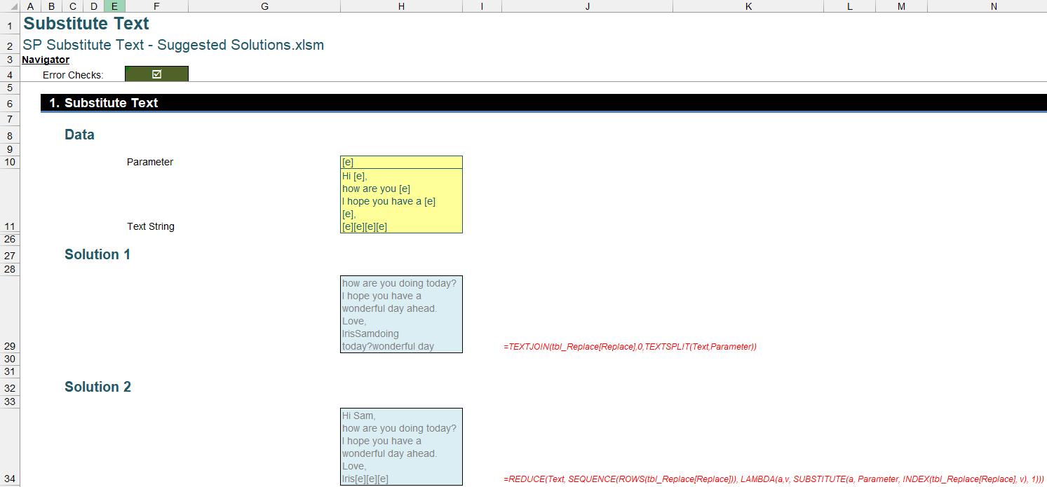
You were given a text string with multiple occurrences of the placeholder '[e]' and a replacement table that provides different replacement values for each '[e]'.  The main goal was to create a dynamic solution that replaces each '[e]' in the text string with the corresponding value from the replacement table.  You could download the original question file here.

As always, there were some requirements:

• the formula needed to be within just one [1] column (no “helper” cells)
• you needed to ensure the solution was dynamic so that it updated when new placeholders or replacement values were added
• no VBA or Power Query was allowed; this was purely a formula challenge.

Suggested Solution 1

You can find our Excel file here, which shows our suggested solution.  The steps are detailed below:

Splitting and Joining

The main idea is to split the text string by the delimiter '[e]' into multiple parts.  Then, add the replacement values at the end of those parts and join them together to create a new text string that satisfies the requirements.

In the Excel file, we have named Text as the text string value, Parameter as the placeholder value, and tbl_Replace refers to the replacement table.

1. SPLITTING THE TEXT

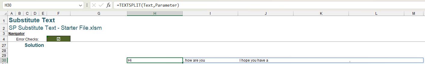
We use the TEXTSPLIT function to split the text string into multiple parts:

This formula creates a dynamic array that spills to the right.

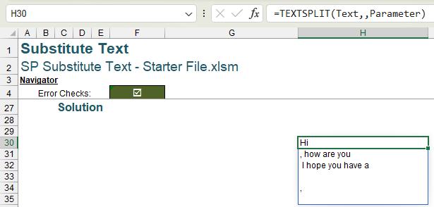
For easier visualisation, we change the formula to make it spill down:

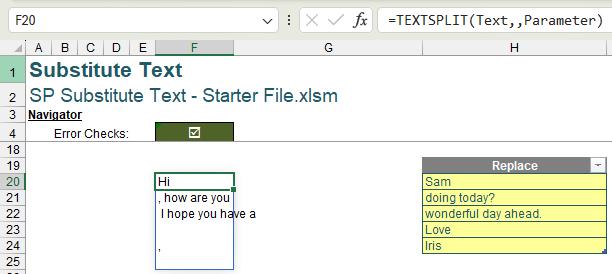
Placing this side by side with tbl_Replace:

2. JOINING THE TEXT

At this point, we use the TEXTJOIN function to join everything together:

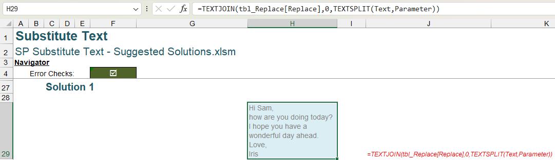
This will give us the desired solution.

Suggested Solution 2

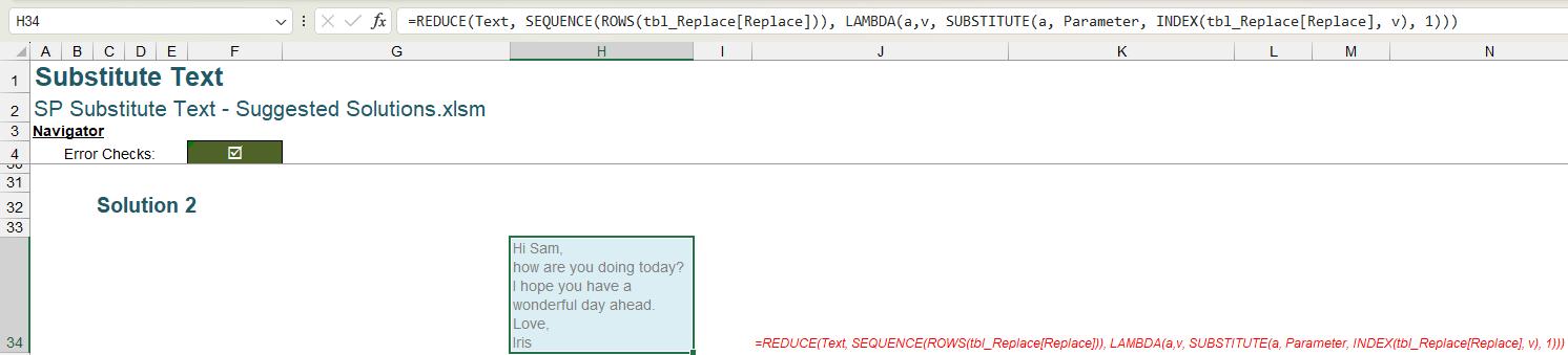
We can achieve the same result using multiple iterative formulas with the SUBTITUTE function.  To replicate the action above in one formula, we can use:

This works as follows:

• SEQUENCE(ROWS(tbl_Replace[Replace])) creates an array from one [1] to the number of replacements we have
• INDEX(tbl_Replace[Replace], v) picks up the suitable replacement value
• the REDUCE function acts as a For Each loop, like VBA.

The picture below illustrates the process of REDUCE getting the result with each iteration:

Word to the Wise

There are some differences in the results of Solution 1 and Solution 2.  If there are more placeholders than replacement values:

• Solution 1 will loop back to the first replacement value
• Solution 2 will keep '[e]'.

We appreciate there are many, many ways this could have been achieved.  If you have produced an alternative, radically different approach, congratulations – that’s half the fun of Excel!

The Final Friday Fix will return on Friday 30 August 2024 with a new Excel Challenge.  In the meantime, please look out for the Daily Excel Tip on our home page and watch out for a new blog every business working day.