
Monday Morning Mulling: June 2024 Challenge
1 July 2024
On the final Friday of each month, we set an Excel / Power Pivot / Power Query / Power BI problem for you to puzzle over for the weekend. On the Monday, we publish a solution. If you think there is an alternative answer, feel free to email us. We’ll feel free to ignore you.
The Challenge
Usually, we position our challenges so that they are accessible to all – but this month (sorry!), we decided to create a test that perhaps not everyone was able to play with. We procrastinated on this one, but felt that the recent introduction of the regular expression (“regex”) functions had presented a possible issue some of you will want to overcome. Therefore, we felt this challenge was both apt and timely. For those who weren’t able to play, don’t worry, normal service will resume next month!
Regular expressions (“regex”) is a language used for pattern-matching text content and is frequently implemented in various programming languages such as C, C++, Java, Python, VBScript – and now, Excel.
Perhaps we need to learn a little about “regular expressions” before continuing. Alternatively referred to “rational expressions” upon occasion, a regular expression is a sequence of characters that specifies what is known as a “match pattern” in text. You have most likely used this functionality in Excel already, with features such as “Find and Relace” or by using the FIND or SEARCH functions in Excel. The purpose of these three [3] new functions (presumably, this is just a start!) is to help you match, locate and manage text (strings) in Excel.
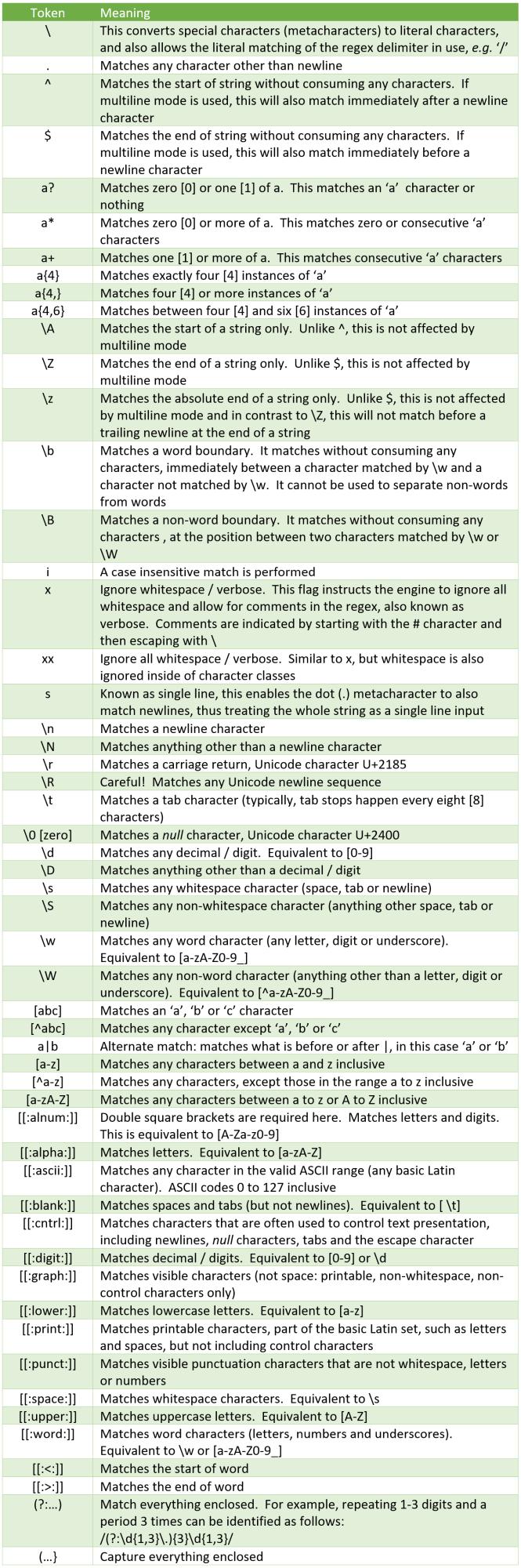
The text is obvious but understanding patterns requires you to learn the syntax for regular expressions. Here is a crash course table, which summarises some – but not all – of the main elements, usually referred to as “tokens”.
This month’s challenge revolved around one of the new functions: REGEXEXTRACT.
This function is used to extract one or more strings that match a specified pattern from the text being analysed. You may extract the first match, all matches or capturing groups from the first match. Its syntax is as follows:
REGEXEXTRACT(text, pattern, [return_mode], [ignore_case])
It has the following three arguments:
- text: this is required, and represents the text you are searching within
- pattern: this is also required. This is the regular expression to be applied
- return_mode: the first of two optional arguments, this specifies which matches to return. It has three alternatives:
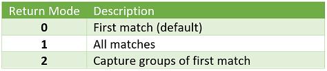
- Capturing groups are part of a
regular expression (“regex”) pattern surrounded by parentheses “(…)”. They allow you to return separate parts of a
single match individually
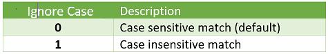
- ignore_case: the final (optional) argument. This determines whether the match should be case sensitive. It has the following two [2] options:
This function always returns text values. You may convert these results back to numerical values using the VALUE function.
The attached Excel file provides examples (and a solution):
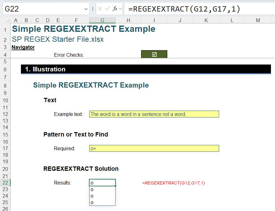
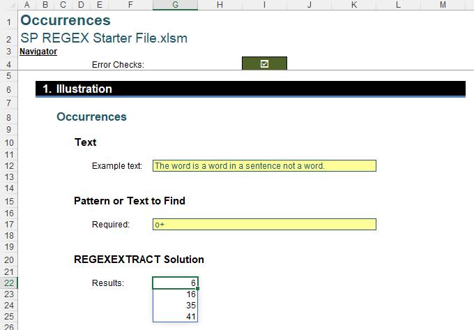
Here, the pattern “o+” (matches one [1] or more of “o”) is defined in cell G17 and extracted from the text string situated in cell G12. There are four instances:
The word is a word in a sentence not a word.
That’s interesting. It might as well tell us there are just four [4] instances. But what if I wanted to know the position of these instances in the text string instead (i.e. the instances of one or more letter “o” texts in a row occurs in positions 6, 16, 35 and 41)?
Let’s keep this challenge simple. I appreciate not everyone is yet conversant with regex syntax, so let’s consider the pattern to be “word” instead, viz.
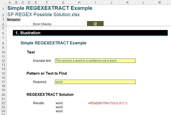
The challenge was to find the position(s) of the text / pattern in the text string:
As always, there were some rules:
- this was a formula challenge; no Power Query / Get & Transform or VBA!
- no helper cell(s) is / were allowed
- the formula should have used REGEXEXTRACT so that regex patterns may be sought and returned.
Once again, apologies to anyone who cannot use this function yet. It is presently being rolled out to the Beta channel. You will need both patience and:
- Windows: Version 2406 (Build 17715.20000) or later
- Mac: Version 16.86 (Build 24051422) or later.
Suggested Solution
To be honest, this isn’t the most difficult challenge we’ve ever posed; it’s more that it’s restricted to so few users presently. There is a well-established technique in Excel to locate the nth occurrence of a character in a text string.
It requires use of the CHAR, FIND and SUBSTITUTE functions, so let’s go through those first…
The CHAR function
Cup of tea? Well a cup of CHAR won’t help you…
This function returns the character specified by a number. You can use CHAR to translate code page numbers you might get from files on other types of computers into characters. Yup, that exciting.
The CHAR function employs the following syntax to operate:
CHAR(number)
The CHAR function has the following arguments:
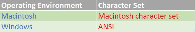
- number: this is required. This is a number between 1 and 255 specifying which character you want. The character is from the character set used by your computer.
For example:
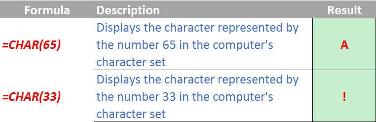
Here, we are going to use CHAR(160) which resolves to "†". This is used because it won't normally appear in text.
The FIND function
The FIND function locates a text “sub-string” inside a longer text string and returns the starting position of it within the parent string (i.e. where the first character is in the longer text string). This function is not available in all languages.
The FIND function employs the following syntax to operate:
FIND(find_text, within_text, [start_number])
The FIND function has the following arguments:
- find_text: this is required and represents the text you wish to find
- within_text: this is also required. This represents the longer (parent) string that contains the text you seek
- start_number: this is optional. This specifies the character at which to start the search. The first character in within_text is character number one [1]. If you omit start_number, then it is assumed to be one [1].
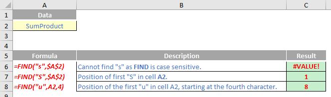
Again, an illustration:
The SUBSTITUTE function
SUBSTITUTE extracts given characters in a string and substitutes other given characters. SUBSTITUTE is similar to REPLACE, but REPLACE requires a specified position to replace a specified number of characters with a given string. SUBSTITUTE replaces one or more instances of a given string within text with a specified replacement string.
Therefore, we might substitute an empty string for all spaces in a string. Often, it is used to leave a 'marker' character in text that allows string manipulation. Its syntax is a follows:
=SUBSTITUTE(text, old_text, new_text, [instance_number])
where:
- text: this is required and represents the text or the reference to a cell containing text into which you want to substitute characters
- old_text: this is also required. This represents the text characters that are to be replaced. It should be noted that SUBSTITUTE is case sensitive
- new_text: also required, this is the text characters that are to be substituted
- instance_number: the only optional argument. This denotes which instance you wish to be replaced. If left blank, every instance of the specified old_text will be replaced by the specified new_text.
For example, a more elaborate use might be
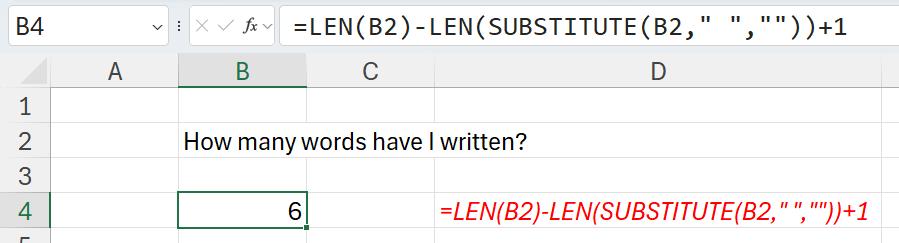
Returning to the Suggested Solution
The three functions may be combined to find the first occurrence of “word” in our text as follows:
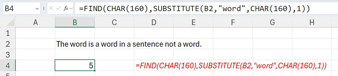
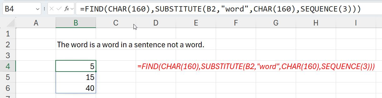
Here, the formula in cell B4 is given by:
=FIND(CHAR(160),SUBSTITUTE(B2,"word",CHAR(160),1))
SUBSTITUTE then replaces the nth occurrence of "word" with CHAR(160). The FIND function then looks for CHAR(160) and returns its position. Given SEQUENCE can be as simple as SEQUENCE(x), which generates a list of numbers in a column 1, 2, 3, …, x, we can use SEQUENCE(3) to find all three occurrences of “word” as follows:
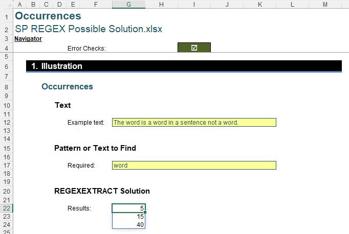
This presupposes we know there are three instances – but we are almost there! The suggested solution to our challenge is therefore the following:
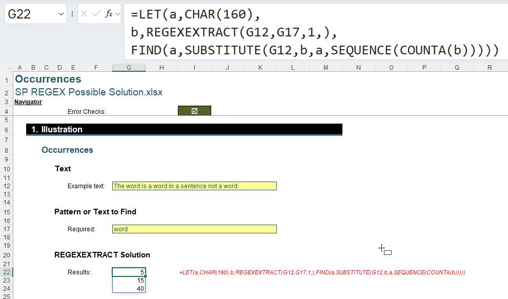
Here, our formula in cell G22 is:
=LET(a,CHAR(160),
b,REGEXEXTRACT(G12,G17,1,),
FIND(a,SUBSTITUTE(G12,b,a,SEQUENCE(COUNTA(b)))))
This is simply using LET to avoid needless repetition of formulae (using internal range names to shorten the formula) and using COUNTA to count the number of occurrences of the text or pattern in order to propagate the TEXT function.
Word to the Wise
We know this month’s challenge was not accessible to all, but we believe the challenge will curb some frustrations with how to use REGEXEXTRACT. No doubt in future Microsoft will unleash a function that will probably provide this result all in one go, but in the meantime…
The Final Friday Fix will return on Friday 26 July 2024 with a new Excel Challenge. In the meantime, please look out for the Daily Excel Tip on our home page and watch out for a new blog every business working day.