Monday Morning Mulling: November 2022 Challenge

On the final Friday of each month, we set an Excel / Power Pivot / Power Query / Power BI problem for you to puzzle over for the weekend.  On the Monday, we publish a solution.  If you think there is an alternative answer, feel free to email us.  We’ll feel free to ignore you.

The challenge this month was to check whether the players unscrambled a set of letters and generate correct words.  Could you make it?

The Challenge

This month, we were playing an Excel word game in which a set of letters was provided, and players needed to unscramble it to make words that have meanings.  Our job as a host was to check whether the words were correctly generated from those letters.

It is easy to check whether a word is meaningful in Excel as we can simply use the Spelling button under the Review tab or press F7.

In this challenge, the objective was to check whether a word was made from the provided letters.  You can download the question file here.

Your solution should have looked like the Check column in the picture below.

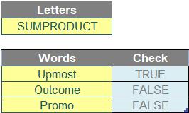
As always, there were some rules:

• this was a formula challenge; no Power Query / Get & Transform or VBA!
• no helper cell(s) was / were allowed
• the formula should not be case sensitive
• the length of words produced by players may vary.

Suggested Solutions

You can find our Excel file here which demonstrates our suggested solutions.  However, before explaining our solutions, we will need to identify what exactly we need to check first.

Brainstorming

There are two points that we need to consider:

1. whether each character of a word exists in the provided set of letters
2. whether duplicated characters in a word are all available in the set.  For example, the word ‘Promo’ in the question has two letters ‘o’ while the letter set ‘SUMPRODUCT’ has only one letter ‘O’.  Hence, this word is invalid.

Returning to the Suggested Solutions

For Excel Office 365, Excel on the Web and Excel 2021:

These Excel versions allow us to use Dynamic Arrays or SEQUENCE function in particular, which shortens a few steps.

Firstly, we can extract each character from a word using the combination of LEN, SEQUENCE and MID as follows.

where:

• List[@Words] refers to the current row on Words column of the List table (@ is known as the implicit intersector and looks for items on a shared row or column)
• LEN counts the number of characters in a string
• SEQUENCE generates a list of sequential numbers from one [1] to the length of the word in an array
• MID helps extract each character from the word, with the starting points from the number series generated above.

Similarly, we use the same method to extract a list of letters.

where Letters is the named range of the provided set of letters.

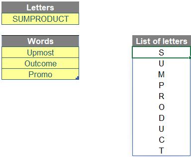
For those of you who use other Excel versions, don’t worry.  We will demonstrate how we may replace this SEQUENCE function with other Excel functions in the next part.

Secondly, we can now start checking the first point as mentioned above, i.e. whether each character in the word exists in the provided set of letters.

There are two common functions in Excel that allow us to rummage through a given text string:

• SEARCH(find_text, within_text, [start_number]) is a search function which is not case sensitive, but does allow for wildcard characters.  It seeks out the first instance of a character or characters (typed in inverted commas) in the within_text text string.  The start_number argument is optional (hence the square brackets in the syntax), so that the first few characters in a text string may be ignored.  If the find_text cannot be located within within_text, the error #VALUE! is returned
• FIND(find_text, within_text, [start_number]) is another search function which is case sensitive, but does not allow wildcard characters.  Apart from that, it works similarly to the SEARCH function.

The third rule of the challenge is actually a hint.  We need to ignore the case sensitivity, which therefore forces us to use SEARCH rather than FIND.  In case an error #VALUE! is returned, we use ISNUMBER to trap the error and return TRUE when it can find a position in the source string.  The formula for the first check is as below:

Finally, we look at the second point, i.e. checking whether duplicated characters in a word are all available in the set.  To count the number of occurrences of a character within a string, we can use the combination of LEN and SUBSTITUTE as follows:

where:

• SUBSTITUTE(text, old_text, new_text, [instance_num]) is used to replace a specific text in a string.  Here, we substitute the characters of each word that exists in the ‘SUMPRODUCT’ set with a blank (“”)
• as SUBSTITUTE function is case sensitive, we apply UPPER function to both words and letters to ignore the case difference between them
• the LEN function helps to calculate the length difference between the original and adjusted words.  This is the number of occurrences of each allowed letter within the words.

Below is an example when we count the number of each allowed letter within the first word (e.g. “Upmost”).

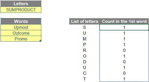
In a similar way, we can use the formula below to count the number of each letter within its set.

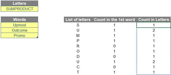
Then, we can check the availability of word characters in the letter set with the condition below:

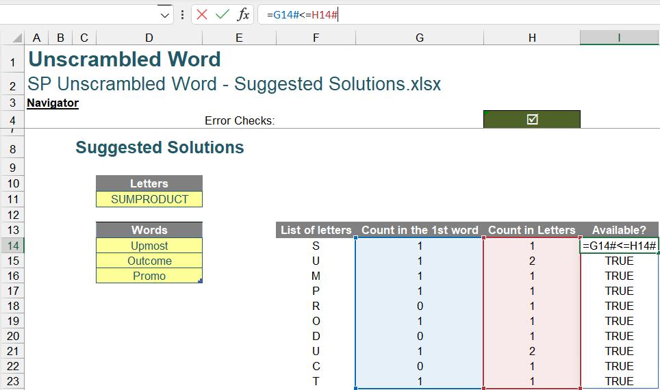
Both existence and availability checks will be combined by AND function as follows:

For all current Excel versions:

We use a similar method as above, except for the SEQUENCE function which may be replaced by the combination of LEN, INDIRECT and ROW functions.  For example, the formula below generates a number list from one [1] to the length of the ‘SUMPRODUCT’ set,

where:

• LEN counts the number of available letters
• INDIRECT converts the range address in text format to a real range, e.g. A1:A10 in this case
• ROW returns a list of row numbers of the range.

Please note that before Dynamic Arrays became available, we had previously written an array formula in what we now call a legacy CTRL + SHIFT + ENTER (CSE) array.  Thus, what is the difference between those two?  The “legacy” CSE array formula requires pressing CTRL + SHIFT + ENTER after completing the formula.  For some formula, we have to select a range for the output and then press the combination CTRL + SHIFT + ENTER whereas the Dynamic Array functions do not require this method of entry.  This is not an issue, but it requires us to visualise the outputs before they are generated so that we select the correct range for the outputs.

Hence, the final formula after replacing SEQUENCE function is as below.

As we know AND function will merge all our arrays into one [1] cell, so we can safely press CTRL + SHIFT + ENTER to get the results.

The Final Friday Fix will return on Friday 30 December 2022 with a new Excel Challenge.  In the meantime, please look out for the Daily Excel Tip on our home page and watch out for a new blog every business working day.