Final Friday Fix: December 2016

Here at SumProduct, we often get asked some pretty tough challenges – the ones that you typically can’t find answers to online. So it pleased us that there was an interesting question that we were asked earlier this month that deserves to appear in our Friday Fix series, and serves as a worthy end-of-year challenge.

Number Formatting

If you’re not aware how you can use number formatting in Excel, you can check out a more comprehensive article here. Suffice to say, we can introduce conditional number formatting into Excel cells using the basic number formatting options, to display numbers such as 10M, 650k and 120 using the same number format, reflecting the values 10,000,000, 650,000 and 120 respectively. We can have no more than three format options in any given cell though.

Our client’s request was to create a cell that would display four different number formats, reflecting billions (B), millions (M), thousands (K) and units. Since we can’t display this in standard number formatting, we are forced to use conditional number formats, with conditions specifying when to apply target number formats.

The Challenge

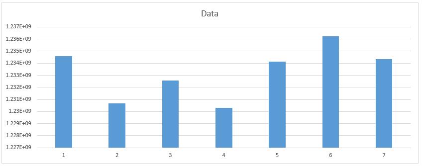
The second part of the client’s request was for the number format to continue onto a chart that the numbers were being reported. Our final Final Friday Fix challenge for 2016 is as follows: can you create a chart to present a row of numbers, where the number format of the chart axis contains 4 or more different conditions? Specific rules:

• It needs to change the number format into billions, millions, thousands or units depending on the numbers presented in the chart (at least 4 different conditions); and
• No macros or user defined functions are allowed.

As always, our solution to the problem will go up next week. Have a good weekend, celebrate the New Year safely, and we’ll see you all in 2017!