Final Friday Fix: October Challenge

Variance Analysis Using Just One Formula

If there’s one thing that can be tedious in Excel, it’s creating a variance report. Imagine you had originally created a budget and as more information came to light, you decided to revise the numbers as follows:

That’s easy enough, right? Put the original budget in the first line and the reforecast data in the second line et voila! you can produce your variance analysis in the bottom row.

But that’s not how management want it. They want it to look like this:

It’s all well and good, but that means a different formula in each cell:

Yuck. That means plenty of opportunities to reference the wrong cell as well as making it impossible to copy the calculation across the row. Thousands of accountants face this thankless task every day – this report can be ridiculously time-consuming and is so easy to calculate incorrectly or misreference. Is there a better way?

The Challenge

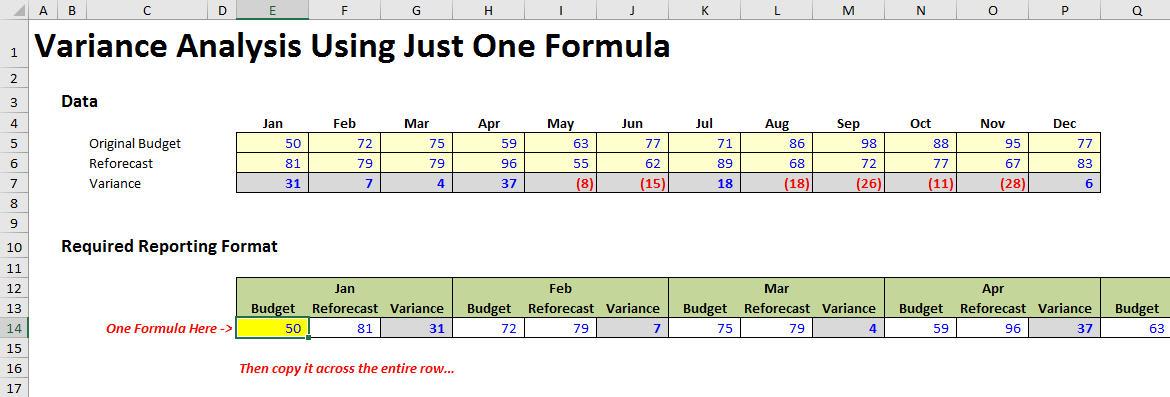
This month’s challenge requires you to download the attached Excel file. Once you open it, you will be presented with the following challenge:

All you have to do is write a formula in cell E14 that can be copied across the entire row of the Report Table. 

Think it sounds easy?  You’ve done this before?  Download the file and give it a shot, because it’s not as straightforward as you might think.  We’ll publish our solution in Monday’s blog.  Have a good weekend, and see you in November!