Monday Morning Mulling: September Challenge

Final Friday Fix: September Challenge Recap

On Friday, we asked you filter the following report so that only values a ‘1’ in the middle digit are reported in the PivotTable.

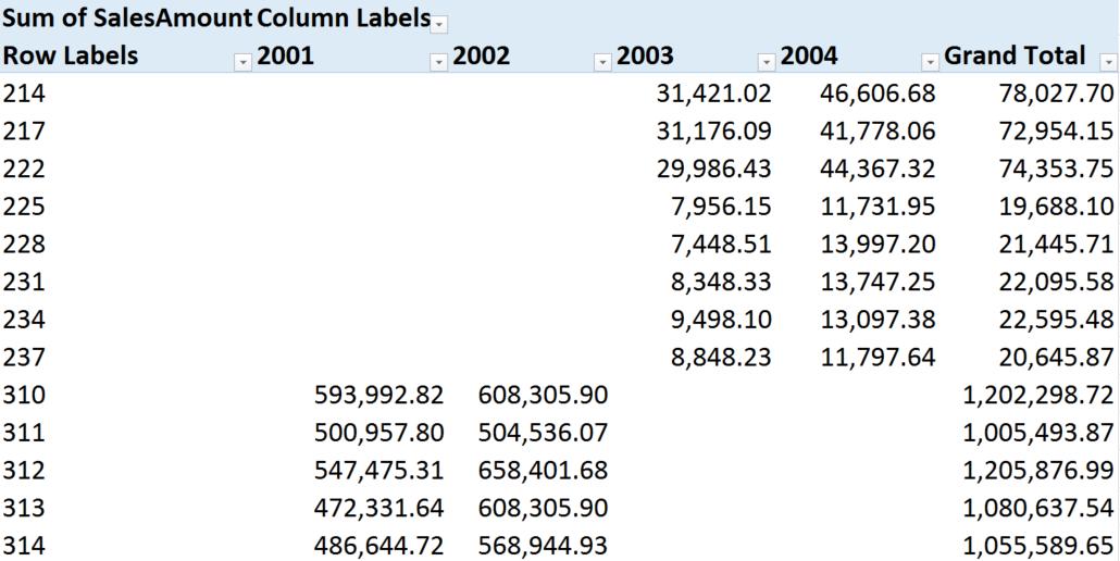
There are two parts to this particular challenge. The first is in understanding how Label Filters work.

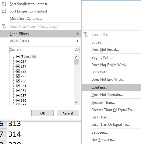
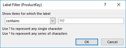
By using the “?” delimiter, we can specify that we want any single character, followed by a ‘1’, followed by another single character, to get our final filtered result:

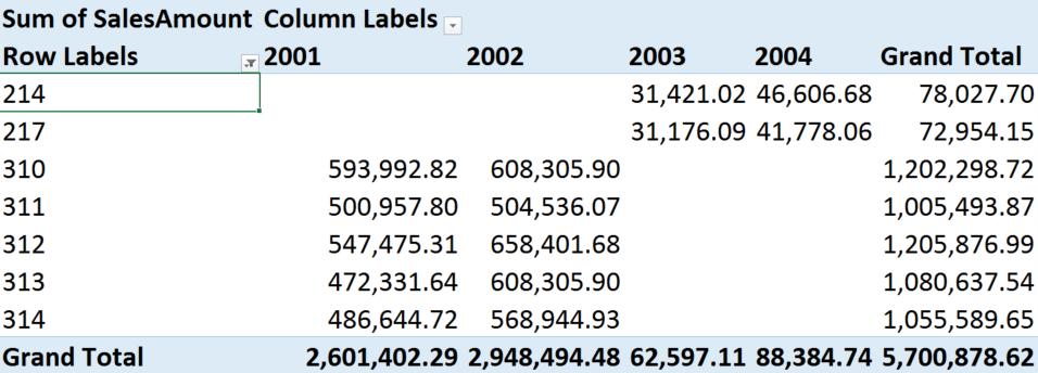
This may have seemed to be the obvious solution to people who have used text labels in the past, and the nice thing is that you can apply this logic to numerical values as well as text ones.

Now, what makes this challenging is that in the Excel file, the Label Filter wasn’t an available option:

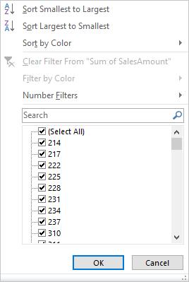
So, what was wrong?

Well, one of the tricks that you can do in Excel is to put what is commonly known as an auto-filter (now just called “Filter”, found in the “Sort & Filter” group of the Data tab) onto a PivotTable. This allows you to filter the results of the PivotTable, which isn’t normally possible using the standard filter options.

However, doing this results in the normal PivotTable row filters being overridden by the “Sort & Filter” filter, which is why in the challenge file, we can filter by color (colour for those of us who spell English correctly J), which we normally wouldn’t be able to do in a PivotTable.

So to solve the problem in this case, it’s as simple as removing the filter from the table, and the PivotTable filters are restored and can be used again.

Fun fact: if you need to keep the Filter in place, but you still want to use the Label Filter, then let me introduce you to a useful shortcut. Alt + Down can generally be used in Excel to pull open dropdown lists, which include filter dropdown menus. Interestingly, even though clicking on the arrow will open the Filter menu, using the shortcut will firstly pull open the PivotTable filter menu first, and only once that’s cancelled or activated, will it then open the Filter menu.

The Final Friday Fix will return on Friday 28 October with a new Excel Challenge. In the meantime, please look out for the Daily Excel Tip on our home page and watch out for a new blog every other business workday.