Power Pivot Principles: Calculating Measures

Welcome back to the Power Pivot Principles blog. This week, we’ll examine an example of how to convert a field to a measure.

If you followed our blog last week, we summarised a budget in Power Pivot. To refresh your memory, here is the summary of that budget, viz.

Before we begin, measures in Power Pivot are Data Analysis Expressions (DAX) formulae that are used for advanced calculations, using various aggregations such as SUM, AVERAGE and COUNT, for those of you wondering. 

Today, we are going to create two simple measures for sales and cost of goods sold (COGS) in Power Pivot, as an example to illustrate today’s subject.  Let’s first look at the Charts of Account sheet and pay special attention to items described as Income and Expenses (Groups P and T in the screenshot) that will be useful in our desired calculations. 

To create a measure, click on Measures on the Power Pivot tab and select ‘New Measure…’

In the dialog box, select the table name Budget and we’ll name our measure ‘Total Sales’.

The next step is to write the DAX code to calculate ‘Total Sales’ and change the Category to Currency:

Using the same steps as above, we will next create another measure for ‘Cost of Goods Sold (COGS)’:

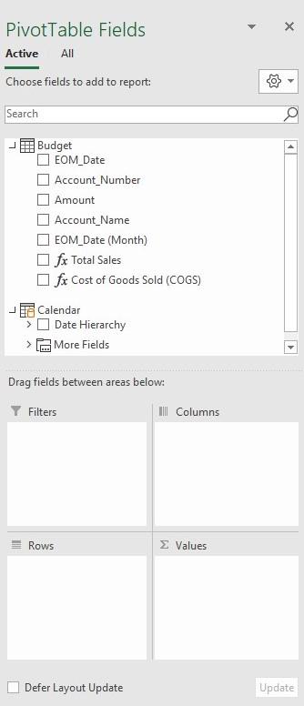
As we can see now, both the calculated measures appear in the ‘PivotTable Fields’ pane.

If we place these measures in the PivotTable, we can get the following result:

That’s it for this week!


Stay tuned for our next post on Power Pivot in the Blog section. In the meantime, please remember we have training in Power Pivot which you can find out more about here. If you wish to catch up on past articles in the meantime, you can find all of our Past Power Pivot blogs here.