Power Pivot Principles: Cumulative Totals with the EARLIER Function
10 September 2019
Welcome back to our Power Pivot blog. Today, we look at another application of the EARLIER function.
Last week we explained how the EARLIER function worked (you can read about it here), and we showed how to use the EARLIER function to create a calculated column that ranks products based on total sale amounts.
This week we’re going to cover another application for the EARLIER function: how to create a cumulative total column in Power Pivot.
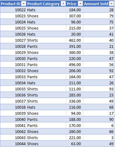
In this example, we will be using the following dataset (this image is not exhaustive):

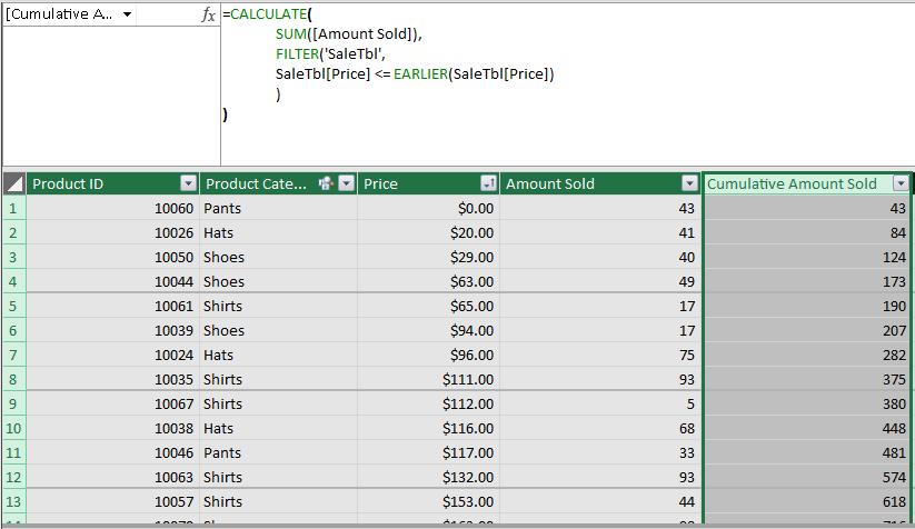
After loading the data to our data model, we may use the EARLIER function to create a cumulative total column. For example, say we wish to write a DAX formula that can calculate the cumulative amount sold for each product, ascending with the price. The formula would look like this:
=CALCULATE(
SUM([Amount Sold]),
FILTER('SaleTbl',
SaleTbl[Price] <= EARLIER(SaleTbl[Price])
)
)

This formula uses the same logic that we covered in the previous blog regarding the inner and outer row context. To avoid repeating ourselves, we will only go over it briefly here:
- The FILTER function is evaluating the Price for each row for the entire table, inner row context
- The function then has to evaluate ‘EARLIER(SaleTbl[Price])’. The EARLIER function instructs the function to evaluate the outer row context which is just ‘SaleTbl[Price]’. On the first row, this evaluates to ‘$0.00’, which is the price of the first row
- The FILTER function then returns with a table with all of the rows that have a price that is greater than or equal to ‘$0.00’
- The CALCULATE function then sums the Amount Sold for all of these rows which is incidentally 43 (in the first row)
- Steps 1 to 4 are repeated for the rest of the rows in the table.
If you are still confused as to how this works, we’d recommend reading our previous blog as go over how the EARLIER function works in greater detail.
Let’s see if the EARLIER function works with dates too.
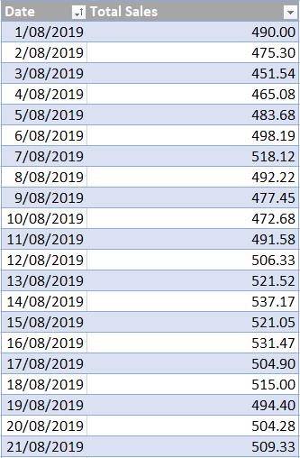
We will be using the following dataset:

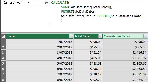
We can use the following DAX code to create a calculated column:
=CALCULATE(
SUM(SaleDataDates[Total Sales]),
FILTER('SaleDataDates',
SaleDataDates[Date] <= EARLIER(SaleDataDates[Date])
)
)

The EARLIER function works with dates too!
That’s it for this week, come back next week for more Power Pivot. Until then, happy pivoting!
Stay tuned for our next post on Power Pivot in the Blog section. In the meantime, please remember we have training in Power Pivot which you can find out more about >here. If you wish to catch up on past articles in the meantime, you can find all of our past Power Pivot blogs here.

