Power Pivot Principles: Introducing ALL

Welcome back to our Power Pivot blog.  Today we discuss how to use the ALL function in DAX.

In Power Pivot, the ALL function returns all of the records in a table, or all of the values in a column ignoring any filters that might have been applied for the filed under scrutiny.  This function is useful for clearing filters and creating calculations on all rows in a given table.

This blog will expand upon the CALCULATE function, first introduced in this blog.  Let’s take it further.  Here, I am going to create a simple ‘All Months Sales’ measure:

Our resulting PivotTable will look something like this:

What next? It sort of stands out doesn’t it? From the CALCULATE and ALL functions, I can now combine them to create a percentage sales measure which will reflect the inherent seasonality (well, for the last six months anyway):

Remember to include an error trap (you can read more about error traps in this blog).

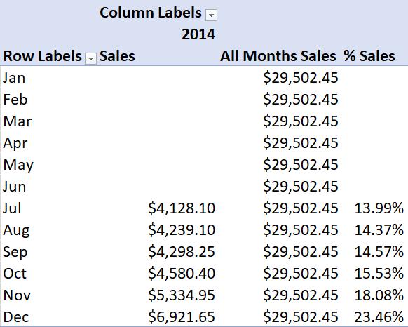
Our PivotTable should look something like this now:

Not only is this percentage calculated from 2014’s total sales, this measure will always be a percentage. This is subtly different from a normal PivotTable, where percentages may be viewed by changing the Value Field Settings rather than an absolute (dollar) amount. Since this measure is based on a month’s sales divided by all months’ sales, this figure will remain a value between zero and one no matter how it is formatted or displayed.

That’s it for this week, stay tuned to our blog for more on Power Pivot. In the meantime, please remember we have training in Power Pivot which you can find out more about here. If you wish to catch up on past articles in the meantime, you can find all of our Past Power Pivot blogs here.