Power Pivot Principles: MAXX

Welcome back to our Power Pivot blog.  Today, we discuss how to use the MAXX function.

The MAXX function evaluates an expression for each row in a table and returns the largest numeric value as a decimal number.  The syntax of this function is:

This means it is useful when you are trying to avoid creating an additional column in a Table to calculate the interim calculations.

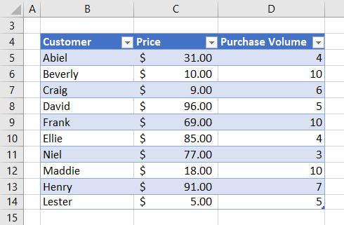
For our example, let’s look at the following Table: 

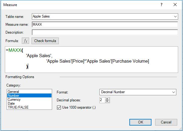
To demonstrate, let’s create a measure using the MAXX function to calculate the greatest amount spent on apples. The expression here is a simple multiplication of ‘Apple Sales’[Price] and ‘Apple Sales’[Purchase Volume]:

In other words, for each row, it is calculating the product of the price and the purchase volume, and then deducing which row creates the highest multiplicative total – all without having to create an extra column for the interim calculation.

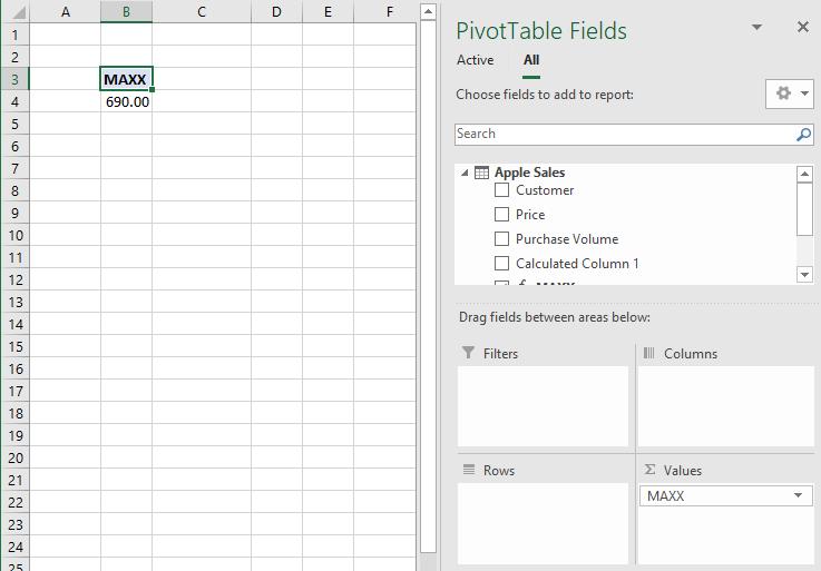
Exporting this to a PivotTable we shall see…:

The greatest amount spent on apples is $690.00.

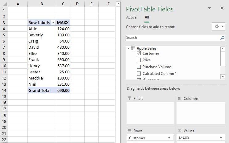
If we drag in the Customer field into the ‘Rows’ area of the Pivot Table:

We can see that Frank spent the most on apples.

That’s it for this week, tune in next week for more on the MAXX function. Happy Pivoting!

Stay tuned for our next post on Power Pivot in the Blog section. In the meantime, please remember we have training in Power Pivot which you can find out more about here. If you wish to catch up on past articles in the meantime, you can find all of our Past Power Pivot blogs here.