Power Pivot Principles: Power PivotTables with Multiple Tables
3 July 2018
Welcome back to our Power Pivot blog. Today, we expand upon our previous blog on PivotTables with Power Pivot.
In our previous blogs we have created PivotTables that filter information for us. However, in those PivotTables we only used information from a single table. As the title suggests, we are going to build a PivotTable from multiple tables.
In Excel it would be very difficult to code a PivotTable to draw data from more than one table; Power Pivot, on the other hand, can do this with ease.
First things first, lets ensure that our dataset has multiple tables. From the ‘Home’ tab in the Power Pivot window we can navigate to the ‘Diagram View’:

We should then see a collection of tables:
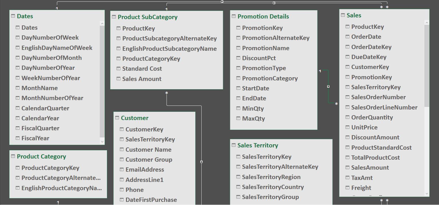
Ensure that the tables have appropriate relationships established, you can read more about establishing relationships here.
Next, head back to our Excel window and look at the PivotTable Fields section:
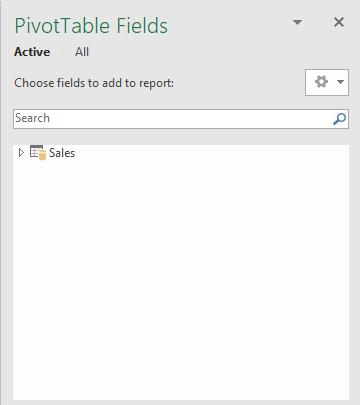
Hang on, there is only one table here, but we’ve linked all of the tables together, they should appear here? This is because we have to select the ‘All’ option (it is annoying that Excel always defaults to ‘Active’, but it is trying to be “helpful”).
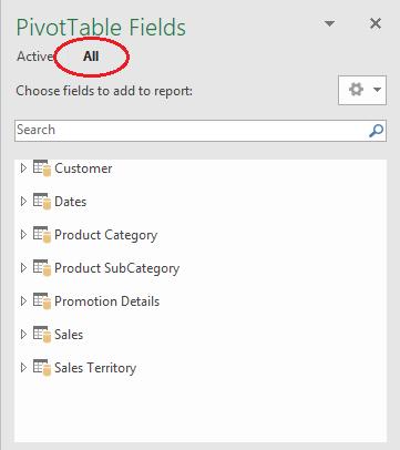
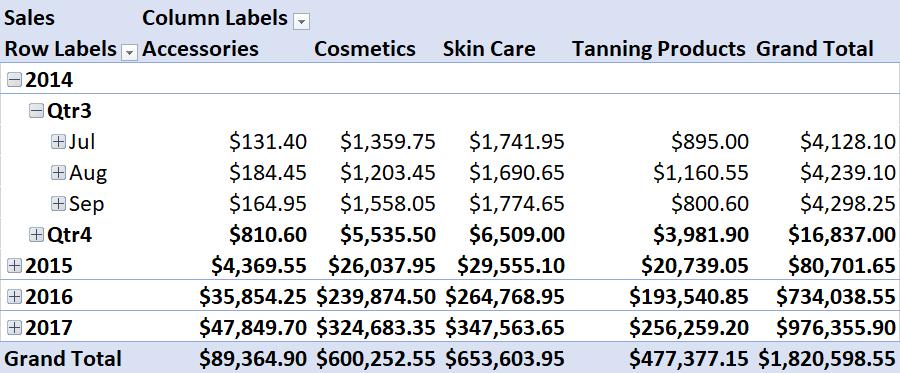
We can create a PivotTable with data from all of the tables in the list here. Let’s start with the Sales from the ‘Sales table’, and the ‘EnglishProductCategoryName’ from the ‘Product Category’ table.
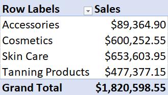
We can also add in the ‘Dates’ from the ‘Dates’ table.

As an added bonus, we can expand on the dates to view the breakdown based on quarters and months:
That’s it for this week, hopefully we’ve taught you something new in Power Pivot.
Stay tuned to our blog for more on Power Pivot. In the meantime, please remember we have training in Power Pivot which you can find out more about here. If you wish to catch up on past articles in the meantime, you can find all of our Past Power Pivot blogs here.

