Power Pivot Principles: Slicers for Columns – Part 1

Welcome back to the Power Pivot Principles blog. This week, we will talk about creating slicers for columns.

To give this idea a context, suppose there is a dataset with Actual revenue

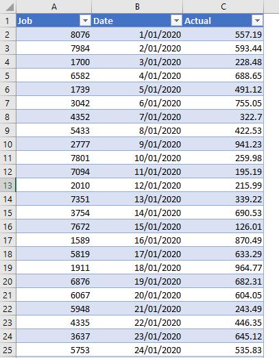
and another data set with Budget revenue for a particular list of jobs.

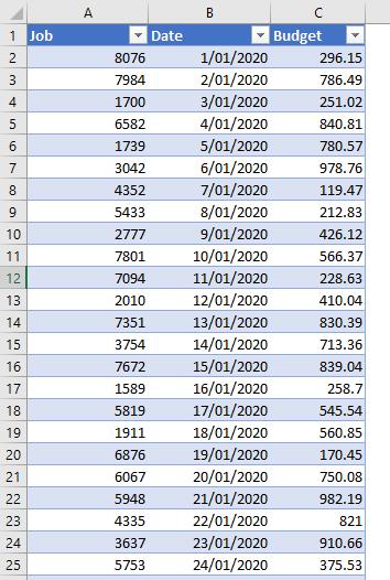
Both tables are loaded into the Power Pivot Data Model.

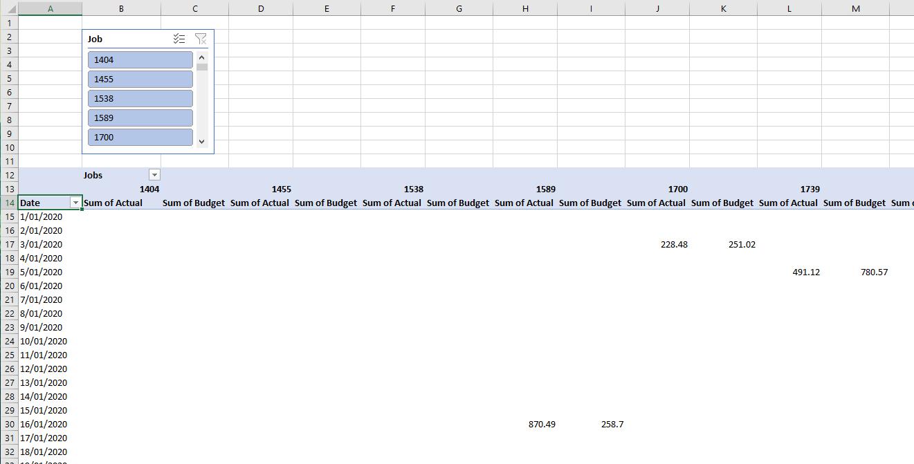
From there, a PivotTable is created with a slicer for the Job field. Each job in the PivotTable includes its Actual and Budget revenue, which are the Value fields and may only be added or removed from the PivotTable Field List. The problem now is that I want to create a slicer, where I can also choose to view either one of Actual, Budget, Variance or all of them.

To do this, I need the help of Power Query to transform my data tables before loading them back into my Power Pivot Data Model. Click on the Actual table and navigate to the Data tab on the Ribbon and choose ‘From Table/Range’.

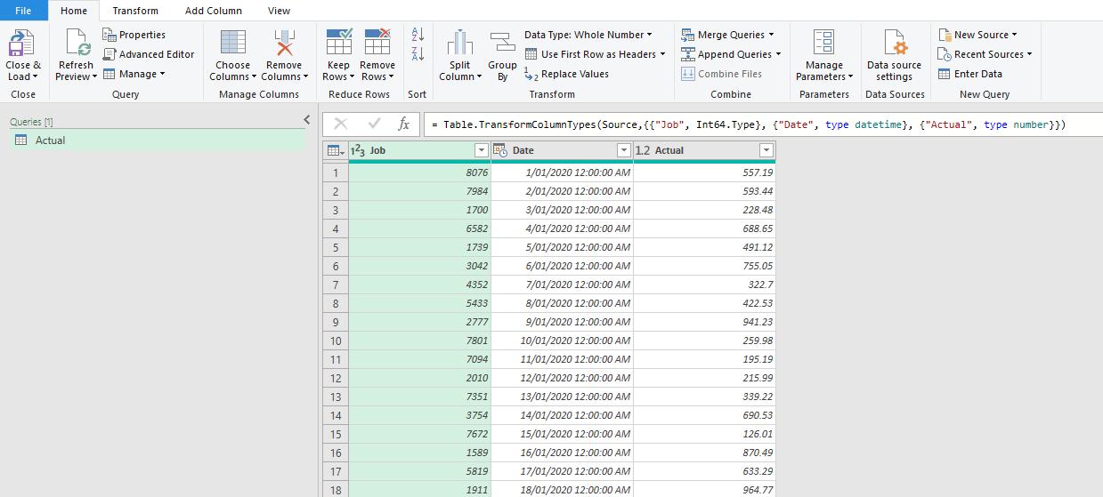
After checking Data Types and ensuring I am happy with field (column) names, I duplicate the Actual table, renaming it to Budget.  I go to the ‘Source’ step, change the ‘Actual’ in the formula bar (or the Advanced Editor) to ‘Budget’.  I do the same with the ‘Changed Type’ step, if necessary.  Since the two tables are in the same structure, this way, I save my time and I do not need to close and load, come back to Excel or go to ‘New Source’ and load the Budget table into Power Query. 

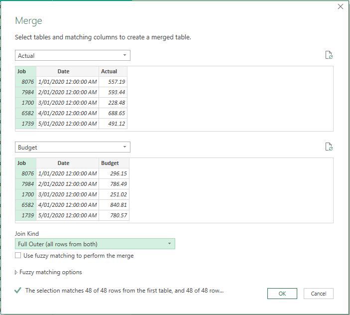
Next, I need both Actual and Budget figures for Job in one table. I go to the Home tab on the Ribbon and select ‘Merge Queries’ -> ‘Merge Queries as New’. The two tables have the Job field in common, the ‘Join Kind’ will be ‘Full Outer’ as I want to take all possible rows from both tables.

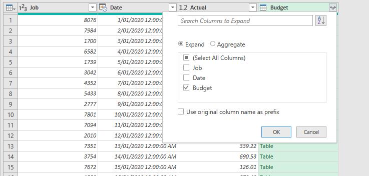
Then, I expand to take the Budget column from the Budget table duly merged.

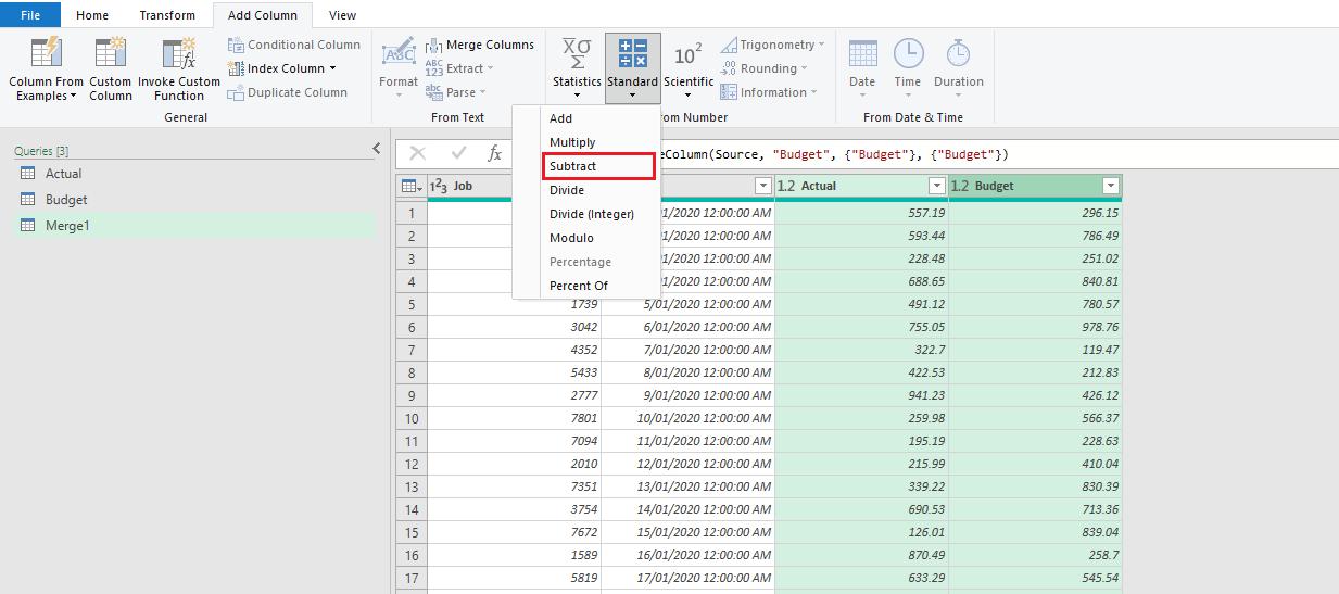
To get the Variance between Actual and Budget, select both Actual and Budget columns, go to the ‘Add Column’ tab on the Ribbon, select Standard -> Subtract.

Next, select the Job and Date columns, navigate to the Transform -> Unpivot Columns -> Unpivot Other Columns (this is in case there are additional columns later).

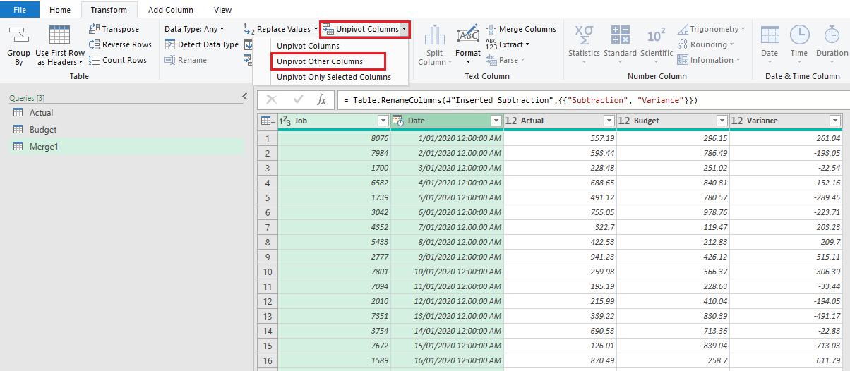
and now the query table should look like the one below:

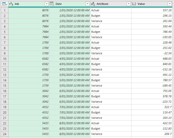
Did you see the light at the end of the tunnel? I will come back next week for the next steps.

Stay tuned for our next post on Power Pivot in the Blog section. In the meantime, please remember we have training in Power Pivot which you can find out more about here. If you wish to catch up on past articles in the meantime, you can find all of our Past Power Pivot blogs here.