Power Pivot Principles: The A to Z of DAX Functions – DB

In our long-established Power Pivot Principles articles, we continue our series on the A to Z of Data Analysis eXpression (DAX) functions.  This week, we look at DB.  

The DB function

The DB function is one of the financial functions.  It returns the depreciation of an asset for a specified period using the fixed-declining balance method.  It has the following syntax:

It has five [5] arguments in the syntax:

• cost: this is required which is the initial costs of the asset
• salvage: this is required which is the value at the end of the depreciation
• life: this is required which is the number of periods over which the asset is depreciated
• period: this is required which is the period for which you want to calculate the depreciation.  The period must use the same unit as life and its value should be inclusive and range between one [1] and life
• month: this component is optional which is the number of months in the first year.  If this argument is omitted, it will be set to the default of twelve [12] months.

There are a few key notes about this DB function

• the declining balance method calculates the depreciation at a fixed rate.  DB function uses the following formulas to calculate depreciation for a period:

• the fixed rate is calculated as follows:

• the DB function will use a different computation for the first [1^st] and the last deprecation:
• for the first [1^st] period the DB function uses this formula:    

• for the last period the DB function uses this formula:

• the period and month are rounded to the nearest integer while the fixed rate is rounded to three [3] decimal places
• an error will occur if:
• cost or salvage < 0
• life, period or month < 1
• period > life
• month > 12.
• the DB function is not compatible with Power Pivot and currently it is only compatible with Power BI, SSAS Tabular, Azure AS and SSDT
• this function is not supported for use in DirectQuery mode when used in calculated columns or row-level security (RLS) rules.

Example

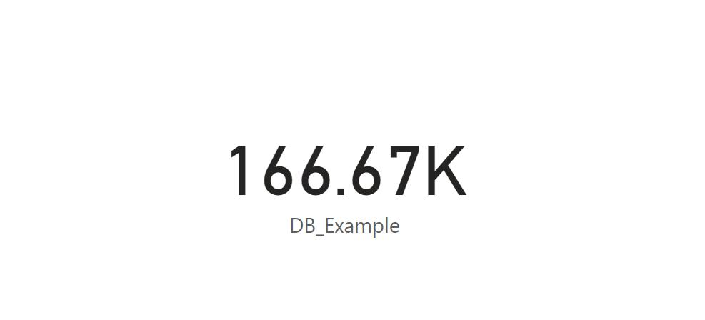
Suppose we have an initial asset that has a value of 1,000,000 and zero salvage value.  The asset has a useful life of six [6] years, and we bought it two [2] months before the current financial year.  Now we want to know the depreciation for the first period.  Hence, I write the following DAX query:

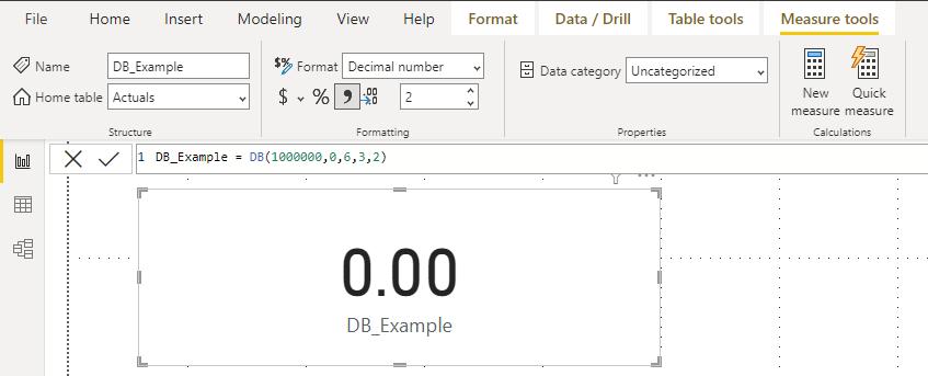
It will have a value of 166,666.67: the declining balance depreciation charge in the first period given that there are two [2] months before the end of the financial year.  However, if you set the period to three [3], a zero [0] value will be returned.  Please see the below demonstration:    

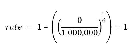
This is because of zero [0] salvage value so the rate will be depreciated at 100% in 12 months:    

In our example, we have two [2] months of depreciation for the first period, giving the number 166,666.67.  For the second period, in ten [10] months’ time, the DB function will depreciate the rest of the asset value.  Therefore, there is nothing left to depreciate for the last two [2] months of the second [2^nd] period and the third [3^rd], fourth [4^th], fifth [5^th] and sixth [6^th] periods. 

Let’s adjust our example to have salvage value of 100,000, the other arguments remain the same as they were in the example above.  Thus, we will depreciate at:

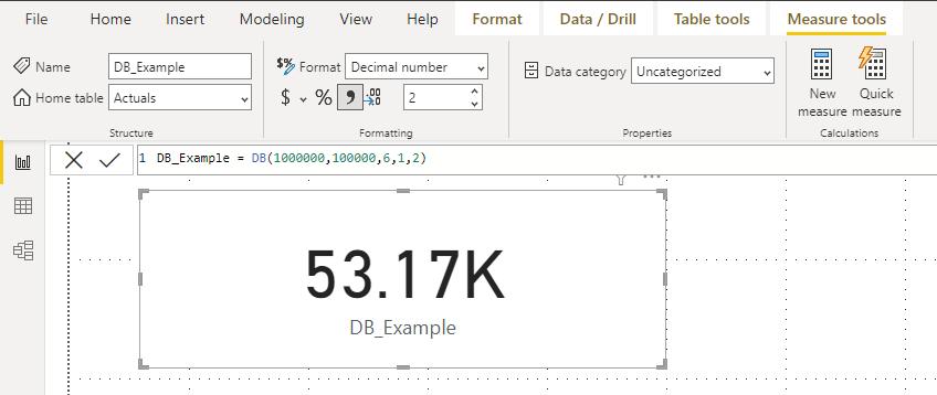
Finally, consider the following DAX query:

It will have a value of 53,166.67: the declining balance depreciation charge in the first period given that there are two [2] months before the end of the financial year. 

Come back next week for our next post on Power Pivot in the Blog section.  In the meantime, please remember we have training in Power Pivot which you can find out more about here.  If you wish to catch up on past articles in the meantime, you can find all of our Past Power Pivot blogs here.