
Power Query: Month Mayhem – Part 3
17 July 2024
Welcome to our Power Query blog. Today, I use the Source Data query as a building block as I continue transforming the data.
My salespeople are back from their break and I have more reports to construct. I have a report with a list of the clients they have been working with each month:
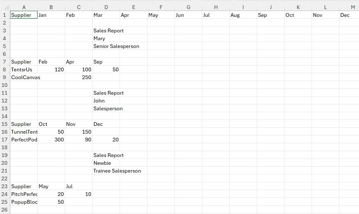
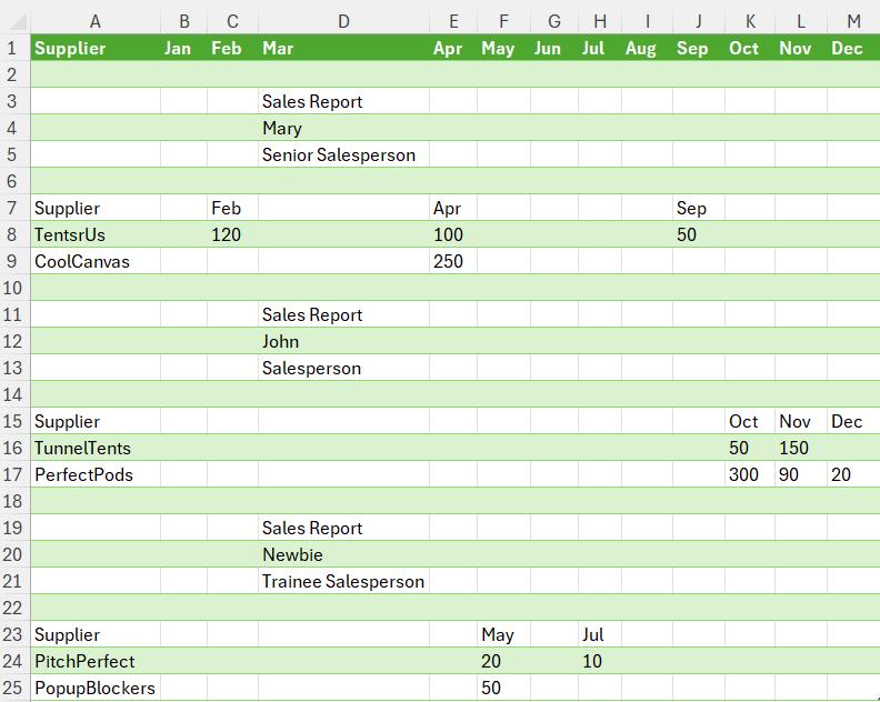
I would like to display the amount details in the salesperson sections but aligned to the relevant month at the top of the page:
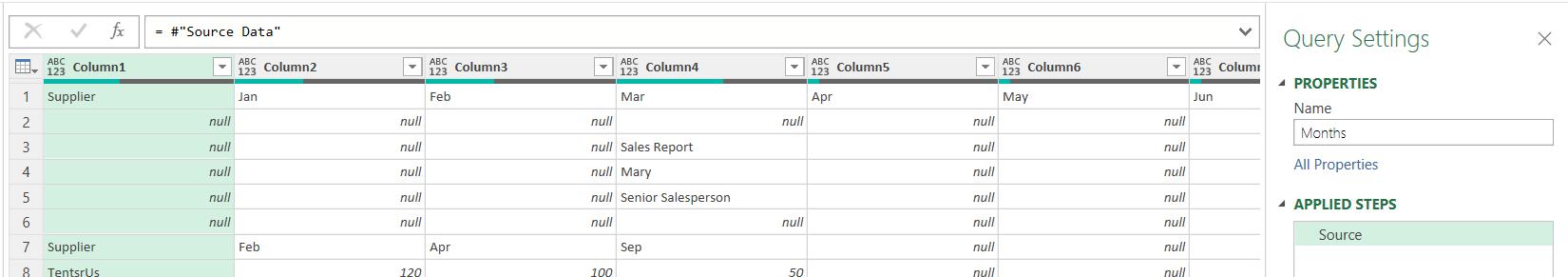
Last time, I completed the Source Data query:
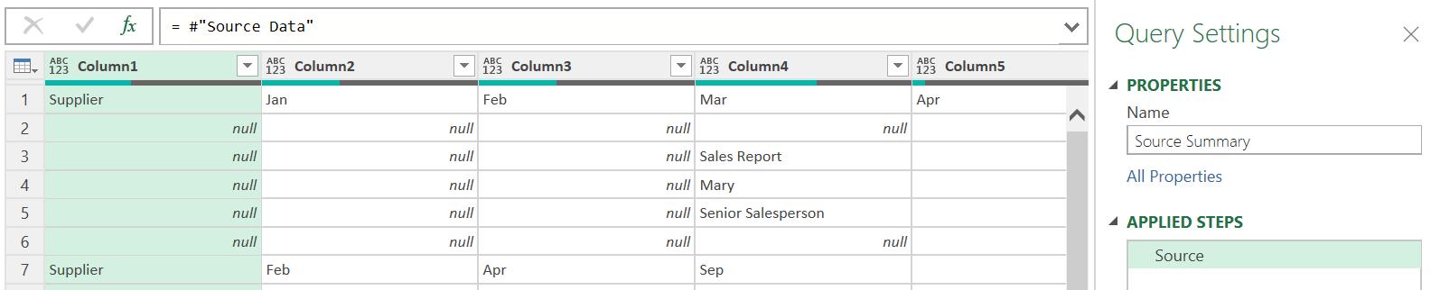
This time, I will take a reference copy of Source Data and continue transforming the data.

I am using a reference copy, as I want the new query to be updated if Source Query is updated, and I don’t plan to change any steps.
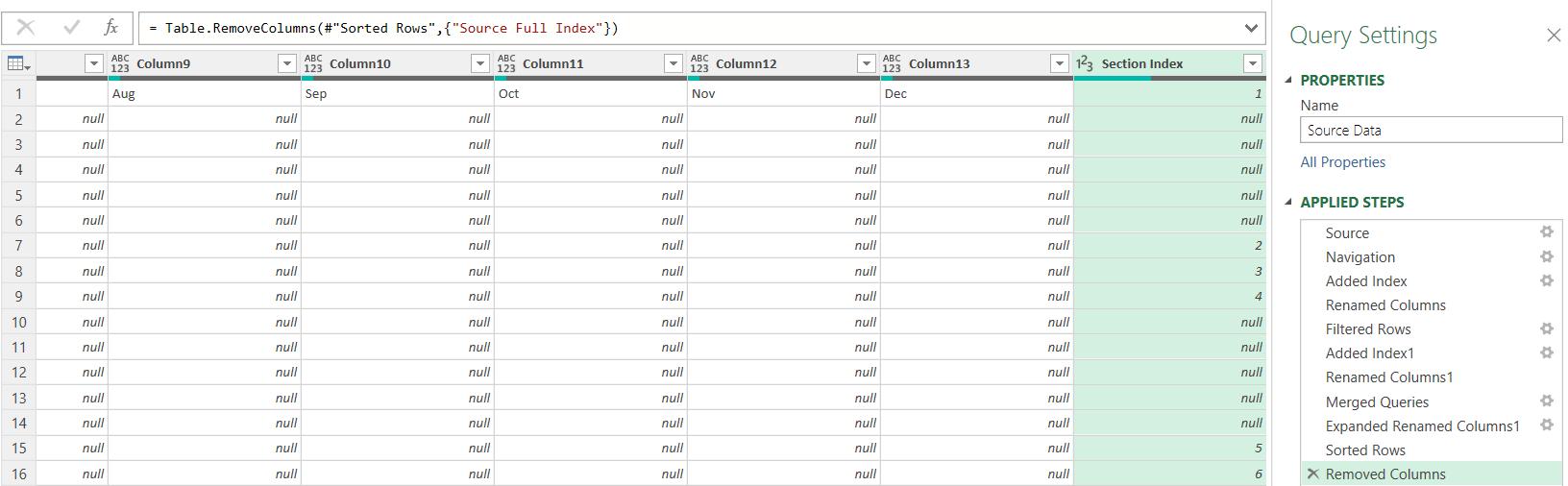
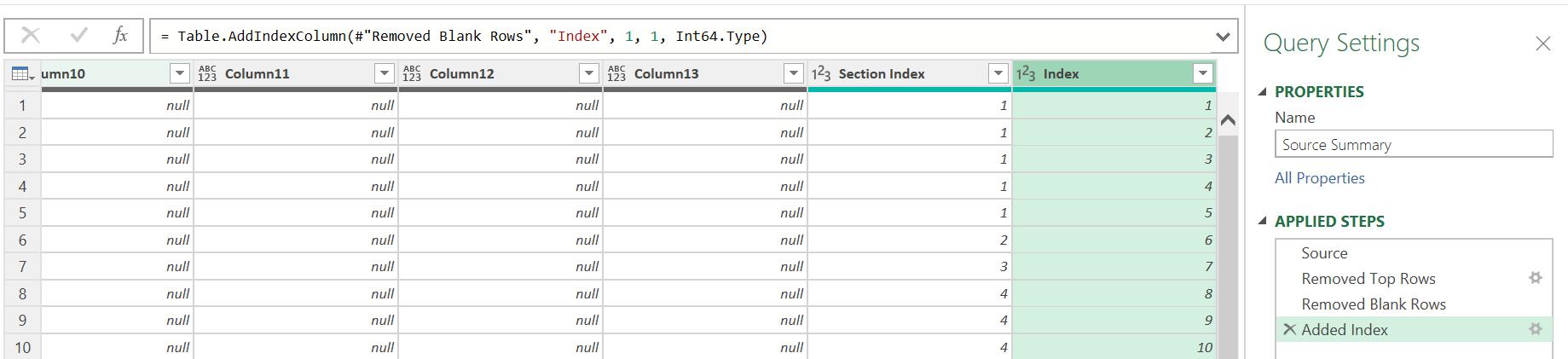
This query will be a summary of the source data at a high level – I call the new query Source Summary:
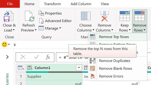
I am going to reduce the rows. I begin by removing the top row, which is the main heading on the worksheet I am transforming:
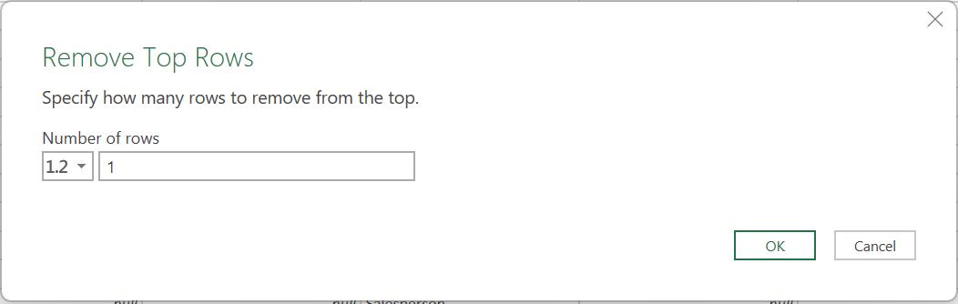
I choose to remove 1 row:
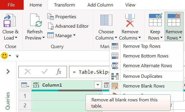
Next, I remove any blank rows:
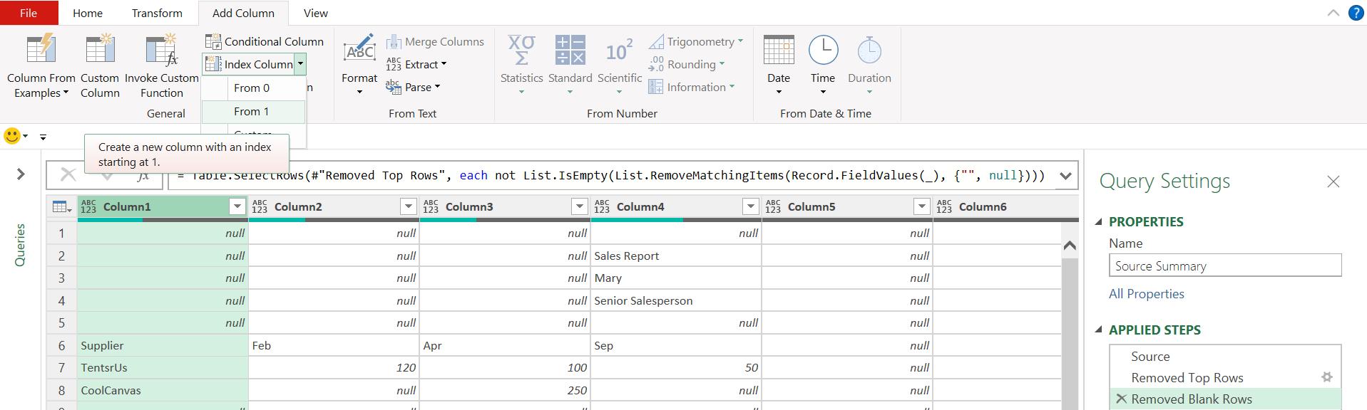
Finally, I add an index from the ‘Add Column’ tab starting from 1. This will help me to identify where my headings go:
My Source Summary query is complete, and I will be using it next week:
I take another reference copy of Source Data and call the new query Months:
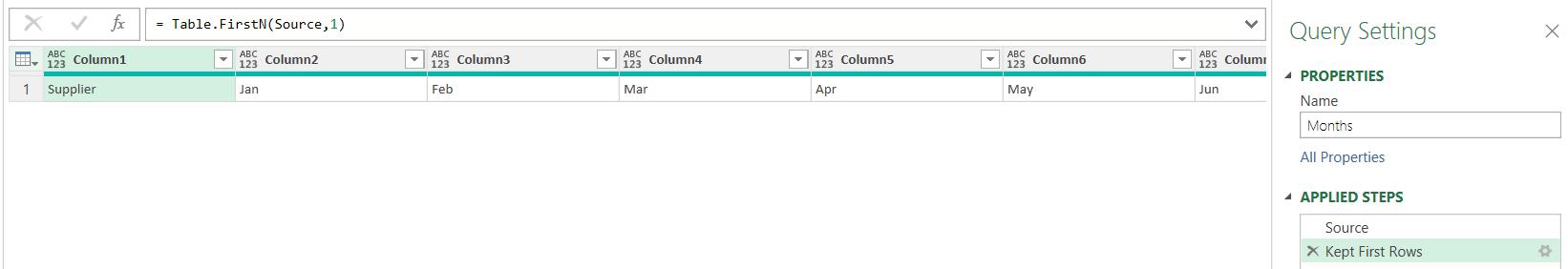
I will need two forms of this query. I start by only keeping the first row. I can do this from the Home tab:
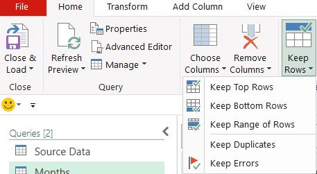
I choose to ‘Keep Top Rows’:
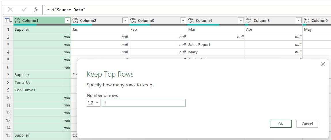
I choose to keep the top row.
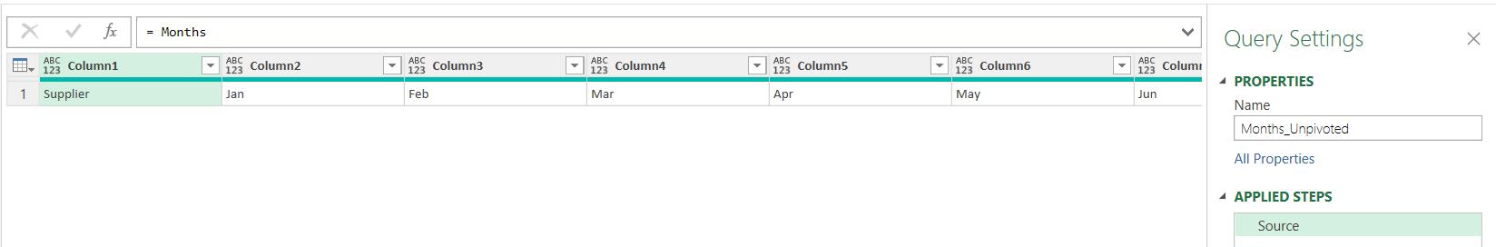
This will be used to merge with other queries. I take a reference copy of this query, which I call Months_Unpivoted:
The purpose of this query, is to get a list of months in a column. I am going to unpivot the data using the option on the Transform tab:
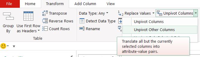
I select Column1 and choose to ‘Unpivot Other Columns’:
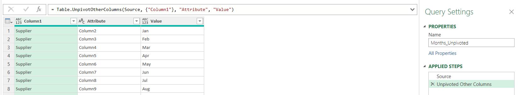
My month queries are ready. Next time, I will create the queries I need for the amount data.
Come back next time for more ways to use Power Query!