Power Query: Skip to the Good Part

Welcome to our Power Query blog. This week, I look at how to remove a random number of rows before useful data.

Yet again, my fictional sales people have been imaginative with their expense forms! I have a form from John, who has decided to add some information that is not necessary for my calculations.

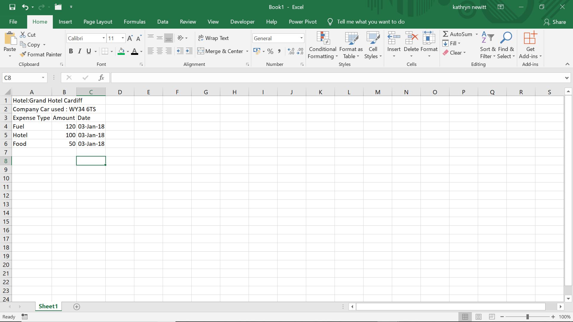
All I need is the expense data – I don’t need to know what car and hotel are involved. However, John likes to use the sheet for any notes that he wants to write and the anount of comment lines may vary. My first step is to create a new query by using the ‘From Table’ option on the ‘Get & Transform’ section on the ‘Data’ tab:

The area of my table is correctly identified, and though I do have headers, they are not at the top, so I leave the ‘My table has headers’ box unchecked.

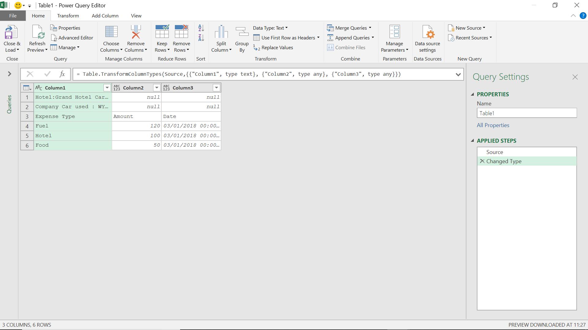
The transformation I am about to perform must work for any number of ‘useless’ rows at the top, so I will need to do more than delete them manually. First, I determine where my header row is. I am going to create an Index column from the ‘Add Column’ tab.

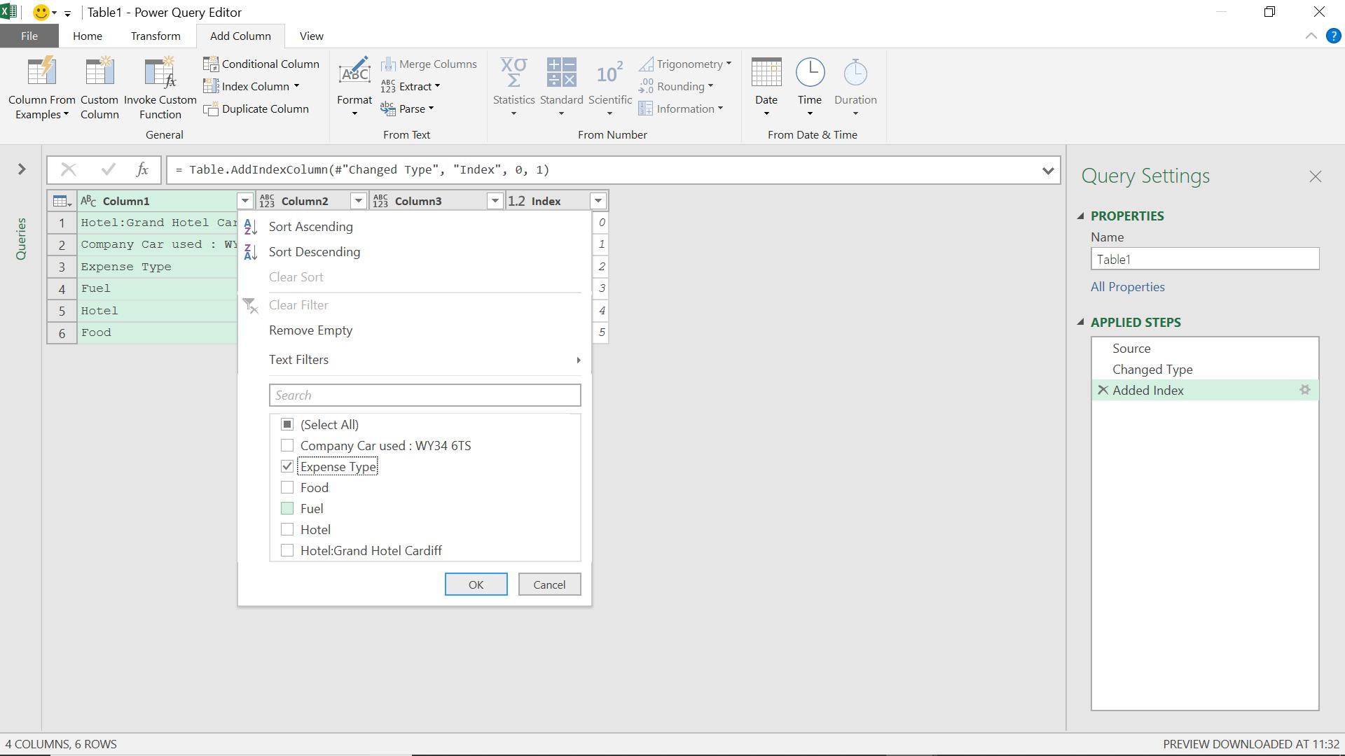
I choose to start at 0, and create my new column:

I filter my data to give me the index number of my header row.

This gives me just the header row. Since Power Query does not change the original data on the Excel worksheet, I can create another source step which points back to my original data.

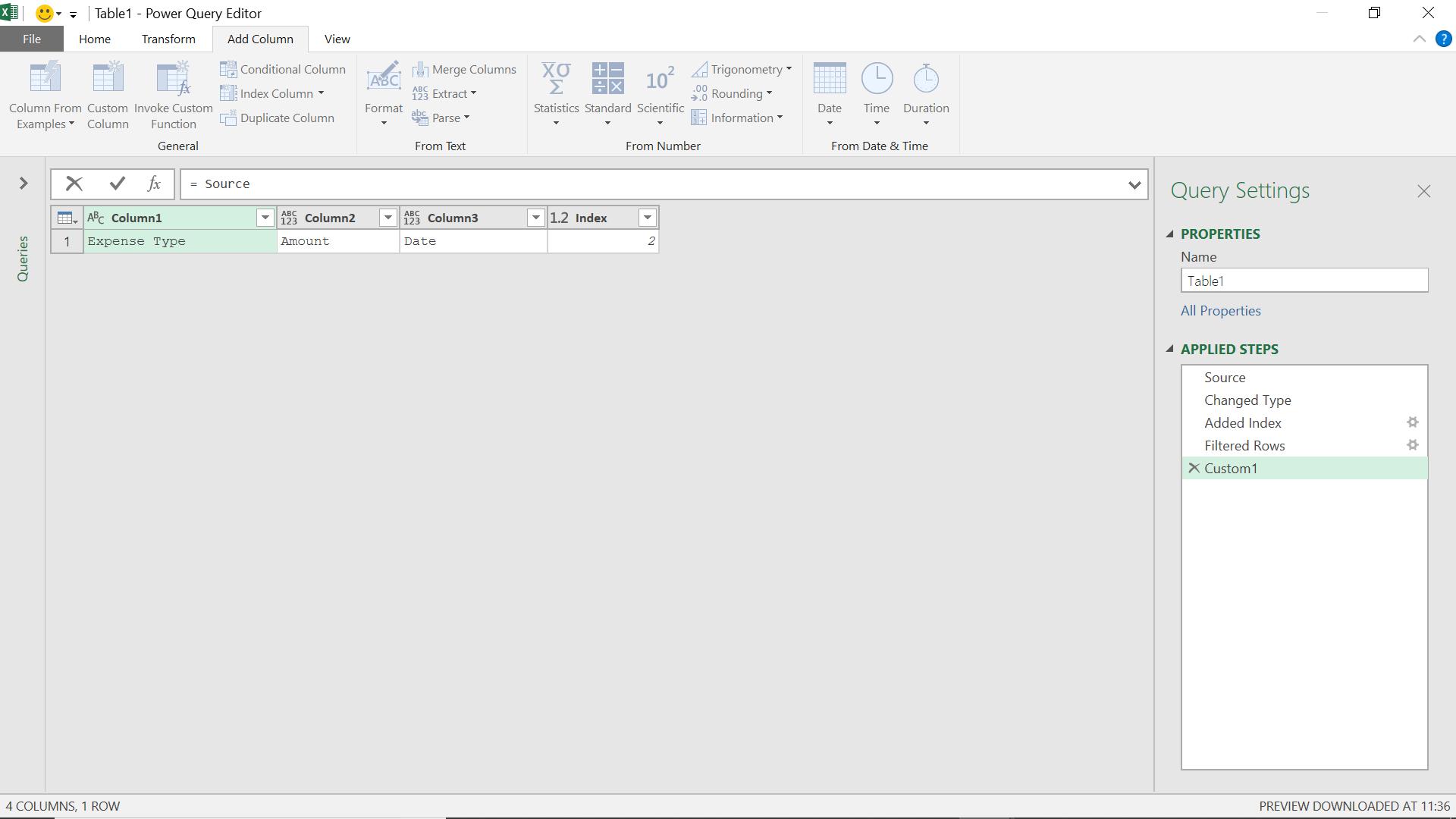
Now I delete my first two rows.  This time, I will manually delete two rows, but next time it could be more or less than that, so this is just the starting point so get at the M code I will need to use. 

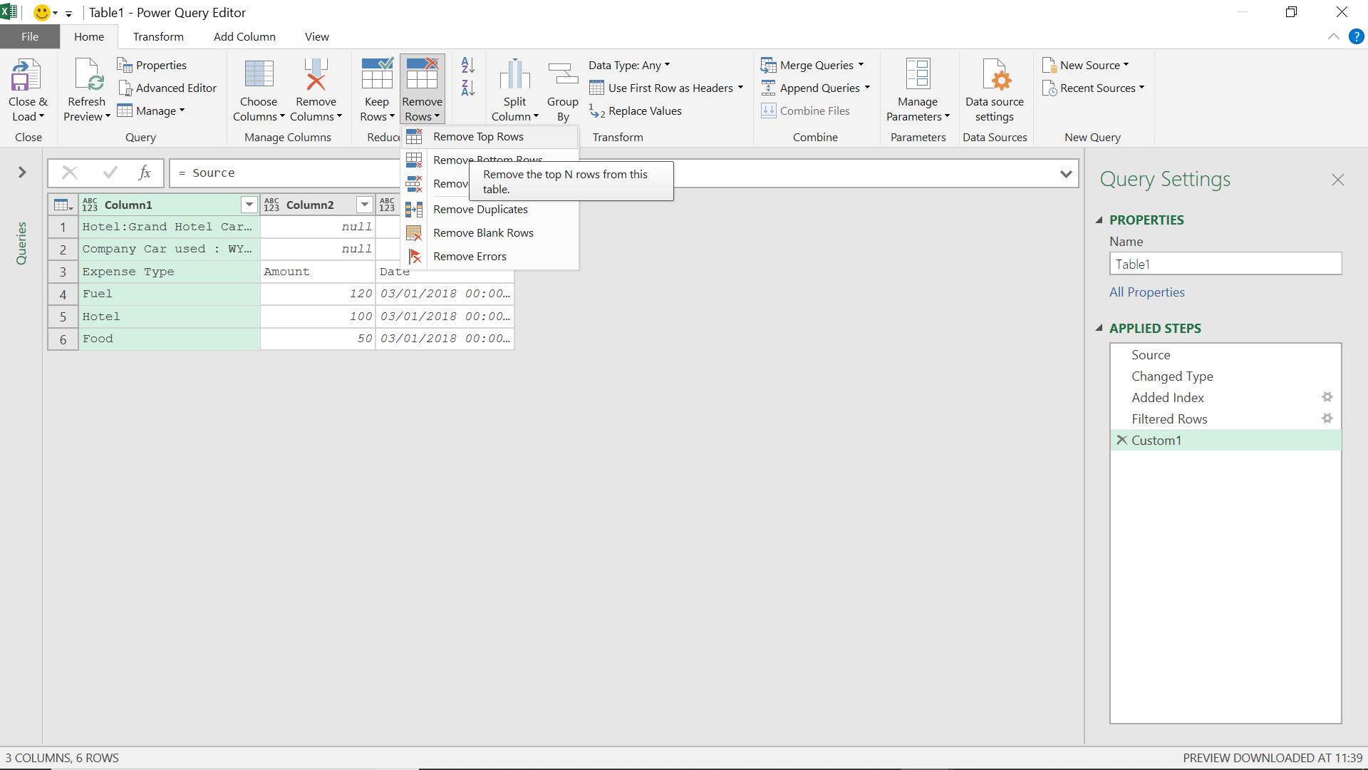
From the ‘Remove Rows’ option on the ‘Home’ tab, I choose to ‘Remove Top Rows’, and for now I will choose to delete two rows.

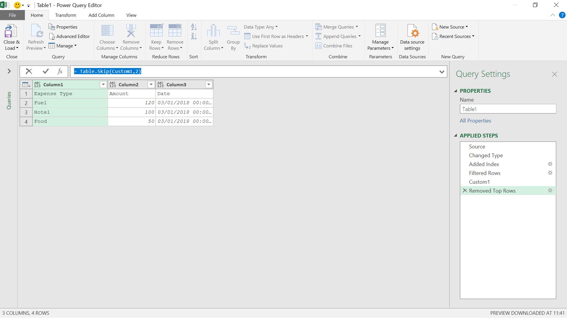
I need to amend the M code for this step to cope with any number of rows.

This is using the M function Table.Skip().

This function returns a table that does not contain the first row or rows of the table. 

where table is the table to modify, and the optional parameter countOrCondition tells the function how many rows to delete. 

Currently, I have a count (2), but I need to amend the Table.Skip() step to use a condition instead, and that condition will be based on the location of my header row.  I need to incorporate my ‘Filtered Rows’ step and use that instead of the value two (2). In order to get the index from the ‘Filtered Rows’ step, I can extract a column from it. 

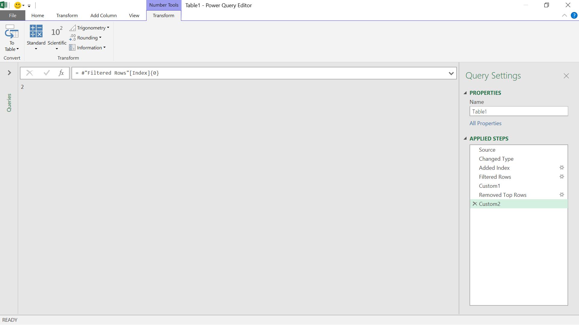
I have extracted the value in the Index column on the first row. To demonstrate why I need the {0}, I can use the function without it to see what I get

I get a list instead of a single value. Using {0} will give me the first value in the list.

Now I have shown how to get the index from the filter step, I can incorporate this into the Table.Skip() function:

My step is now 

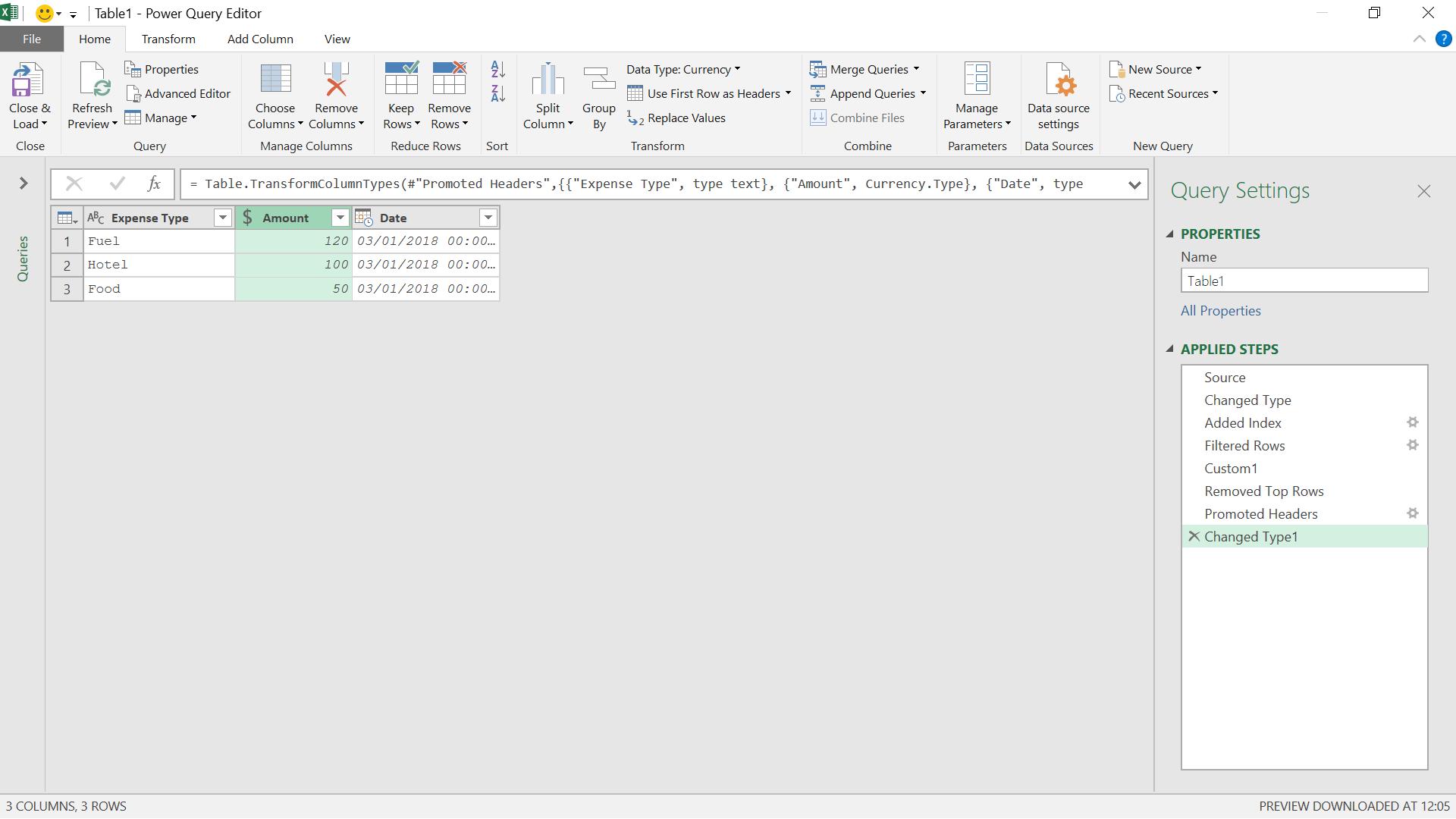
I finish tidying my data ready to test the query.

In order to test my query, I go back to the Excel worksheet and add another line to John’s extra information.

I refresh my query to see what happens.

The source step shows the extra line of information.

My final step has removed all the extra data correctly.

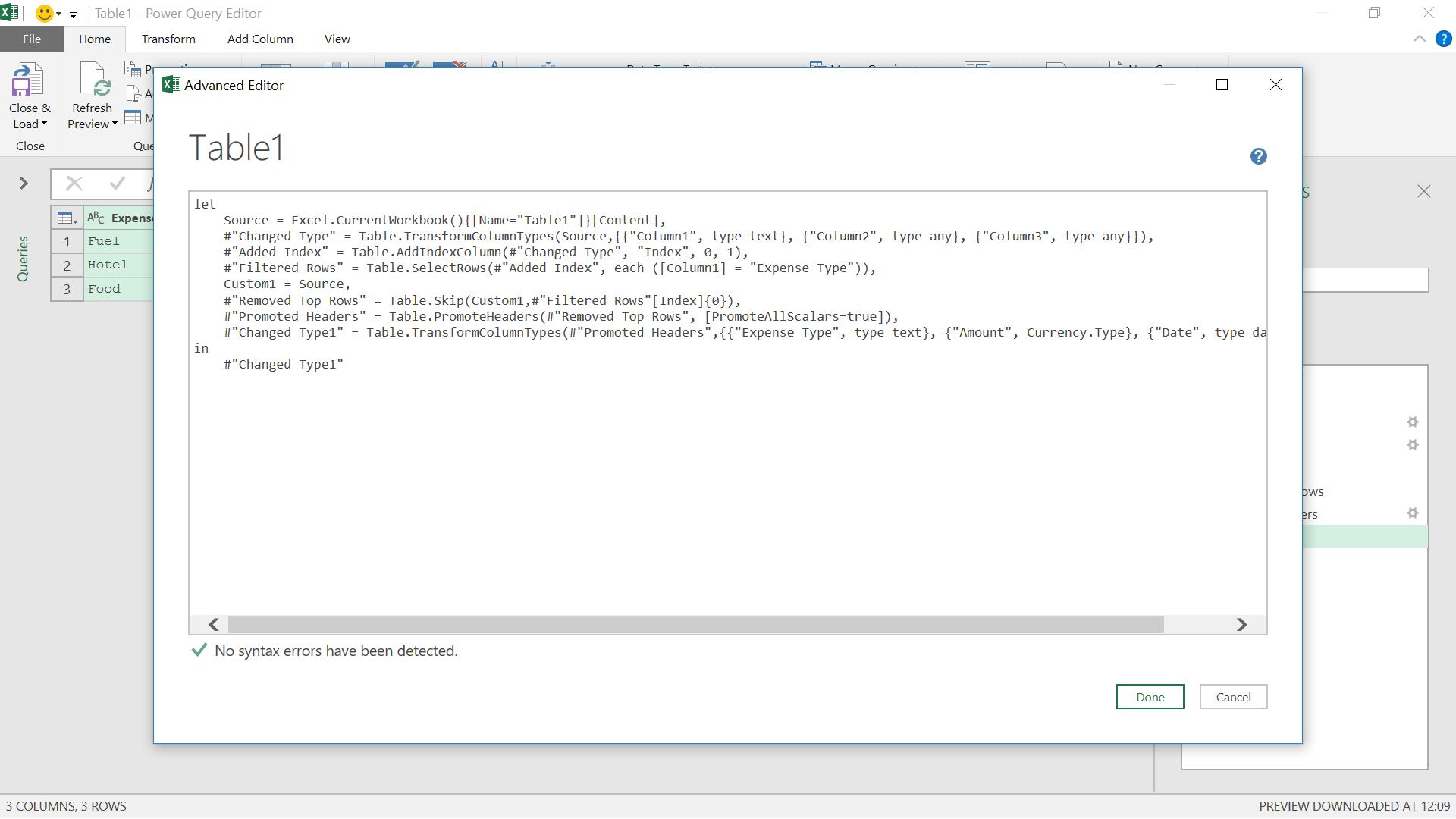
Looking at the M code in the Advanced Editor, I could make a few more changes to make my code more efficient.  I have two ‘Changed Type(n)’ lines that could be combined, and I could also remove the ‘Custom1’ step and point directly at the source in ‘Removed Top Rows’.  However, I know that no matter how much information John decides to share, I can remove it with this query. 

Come back next time for more ways to use Power Query!