Auto Fill Becoming a Drag..?
Had your fill of Auto Fill..? This article looks at an Excel feature that too many take for granted and probably have not explored to its full potential – Auto Fill. By Liam Bastick, director with SumProduct Pty Ltd.
Query
I seem to spend my entire life copying vast lists of data. Any tricks and tips to become more efficient?
Advice
It appears to me that you’re a Luddite in the modelling community if you venture anywhere near the mouse. I have worked with many banking and finance clients that berate staff who have the audacity to let their fingers migrate from the keyboard for even a picosecond.
Therefore, it’s refreshing this month to provide some efficiency tips you can exploit with your furry little friend (and yes, before you all write in, some of the following can be replicated using keyboard shortcuts!).
This article considers Auto Fill.
For those that have not been near a computer in the past 100 years, let me first explain what Auto Fill is. In essence, a cell, or range of cells, is highlighted. Then the mouse is placed over the small black square in the bottom right hand corner and either dragged across or down to fill the intended range. As an example:
Before Auto Fill

Dragged-and-Dropped
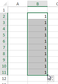
Not without its limitations (e.g. it cannot be dragged down and across simultaneously, moving it upwards / left deletes the contents), it is a highly intuitive tool. Moreover, it is a lightning quick method for copying data down a column.
For example, consider a list with data to be placed in the adjacent column as follows:
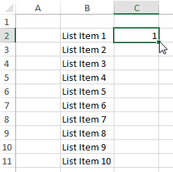
Placing the mouse over the little black square and double-clicking, the column will Auto Fill:
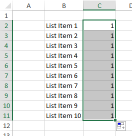
It should be noted that this only works for lists in columns (not rows), but it is a great time-saving device when lists are structured similarly to the above.
So what if Auto Fill seems disabled?
Sometimes, when you click on a cell, or a range of cells, either the little black box does not appear in the bottom right hand corner or else the cell simply will not ‘drag-and-drop’.
In this instance, call up Excel’s Tool Options (ALT + T + O), viz.
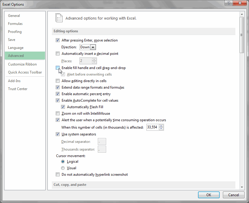
Activate the ‘Enable fill handle and cell drag-and-drop’ check box and drag-and-drop should now work.
So far so good, but I presume most of you will already know this. The thing is, there’s a little more to Auto Fill than this…
More on Auto Fill
In the list of 1’s graphic (above), did you notice the little icon that appeared near the bottom right hand corner of the range? This is the Auto Fill Options icon, and clicking on it, certain options become available:
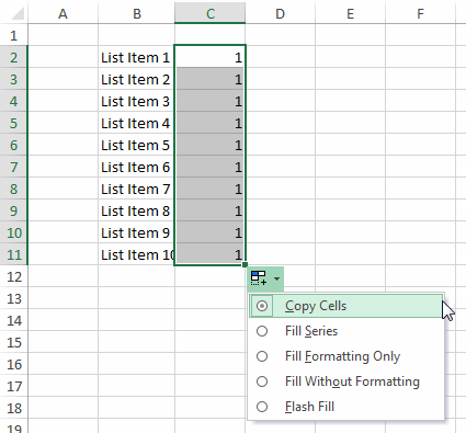
This icon does not appear in all versions and further, not all options are available in all versions of Excel (e.g. ‘Flash Fill’ [see below] is an Excel 2013 feature). If it is absent in your version, have no fear, there is an alternative approach.
Instead of using the left click button of the mouse, use the right click button. Whilst you can no longer double-click to complete a list (see above), dragging down and releasing the button afterwards reveals the following – potentially more detailed – shortcut menu:
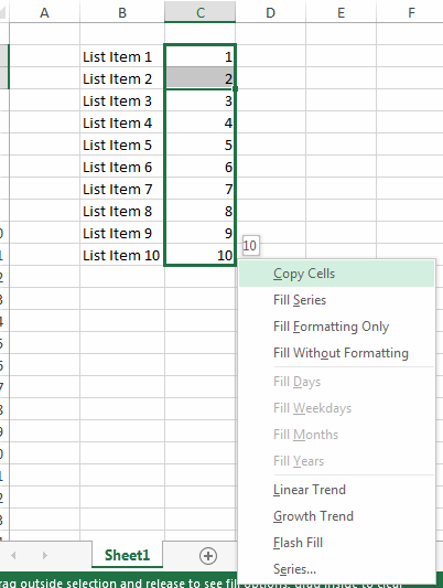
I suspect a lot of users will not be aware of this useful menu, so I will briefly explain what all of the options do:
- Copy Cells: does exactly what it says on the tin, with cells copied in the usual way;
- Fill Series: Excel tries to identify the pattern in your data and extrapolate it. Where Excel struggles, it will often fall back on the ‘Linear Trend’ approach (see below);
- Fill Formatting Only: for those who can’t be bothered to find the ‘Format Painter’;
- Fill Without Formatting: very useful for copying blocks of formulae where the formatting is inconsistent;
- Fill Days / Weekdays / Months / Years: forces Excel to project days (workdays), months and years in the range;
- Linear Trend: Excel assumes the values can be charted on a straight line, using the least-squares algorithm (y = mx + b) to generate the series. Linear regression has been discussed previously (see Trendy Forecasting in Excel);
- Growth Trend: also discussed in Trendy Forecasting in Excel, the starting values are applied to the exponential curve algorithm (y = b*m^x) to generate the series;
- Flash Fill: the flash fill feature is new to Excel 2013 and improves on Excel’s basic pattern recognition, allowing users the ability to pattern fill from one or more text strings to a single column. As an example, consider the following table:
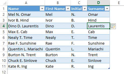
- Column A represents existing data. “Mel” was typed in manually into cell B2 and then the “I” of “Ivor” was typed. The flash fill icon appears (in cell E4 in the graphic) and allows the user to auto fill the rest of the column immediately. Columns C and D were populated similarly.
Clearly, this functionality is aimed at making things easier. However, changing or adding names will not update columns B, C and D automatically, so more sophisticated users may still have to resort to tried and trusted formulaic approaches. It’s a move in the right direction though.
- Series: this option activates another dialog box, viz.
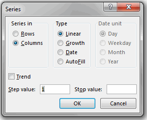
Most of this dialog box is covered by the notes above (rows and columns just allows you to fill either horizontally or vertically, which you can do manually anyway), but here you can generate a trend manually;
If you select ‘Linear’ or ‘Growth’ options (from the shortcut menu), the step and stop values are ignored. However, you can force Excel to extrapolate on your terms.
All you need to do is select the cell where you want to start the series (the cell must already contain a value), then in this dialog box, if ‘Linear’ has been chosen, the step value is added to the first starting value and then added to each subsequent value; if ‘Growth’ is selected, then the first starting value is multiplied by the step value. The resulting product and each subsequent product are then multiplied by the step value;
The stop value is simply the value you want to stop the series at (however, if you Auto Fill a list with data in the column immediately to the left, this stop value may be ignored);
If there is more than one starting value in the series and you want Excel to generate the trend, simply select the ‘Trend’ check box.
Auto Fill with the Control (CTRL) Button
Things vary when the CTRL button is used when dragging and dropping. For example:
| Scenario | Drag-and-Drop only | Drag-and-Drop with CTRL |
|---|---|---|
| Single cell selected, containing a number | Number is repeated in all cells | Number is increased by 1 in each cell |
| Single cell selected, containing text but ending in a number (e.g. “Year 1") | Text is repeated with final number increased by 1 in each cell | Text is repeated in all cells |
| Two cells selected, both containing numbers | Number sequence continues linearly, increasing / decreasing by the difference between the first and second numbers | Pattern will alternate between the two numbers (i.e. numbers are repeated) |
| Two cells selected, containing text but ending in a number (e.g. “Year 1" and “Year 2") | Text is repeated with final number increasing / decreasing by the difference between the first and second final numbers | Pattern will alternate between the two text items (i.e. text is repeated alternately) |
| Single cell selected, containing a day of the week | Day of the week increases sequentially through the range | Same day of the week is copied into all cells |
| Two cells selected, both containing days of the week | Days of the week sequence continues linearly, increasing / decreasing by the difference between the first and second days | Pattern will alternate between the two days of the week (i.e. the days of the week are repeated alternately) |
| Cell(s) containing formula(e) | Will copy normally | Will copy normally |
The problem here is there is not a constant logic; however, with practice, you can soon master these Excel quirks.
Auto Fill with Custom Lists
Why is it that days of the week and months of the year are recognised by Auto Fill? Excel simply recognises they form part of a built-in list. However, you can add your own (custom) lists that may be adopted by Auto Fill too.
To do this, simply do the following:
- Type the required list into contiguous cells in Excel:

- Highlight this list then activate ‘Edit Custom Lists…’. This is a functionality Excel likes to move!
Excel 2003 and earlier
- Go to Tools->Options (ALT + T + O)
- Select ‘Custom Lists’ tab
- Choose ‘NEW LIST’
Excel 2007
- Click the Office button and click Excel Options (ALT + T + O)
- Click Popular’ in the left pane (the default view)
- In the ‘Top Options For Working With Excel’ section, click the ‘Edit Custom Lists…’ button
Excel 2010 onwards
- Click the File tab and select Options (ALT + T + O)
- Select ‘Advanced’ in the left pane
- In the ‘General’ section, click ‘Edit Custom Lists…’
- Once the search party has returned, you will have tracked down the ‘Edit Custom Lists’ dialog box:
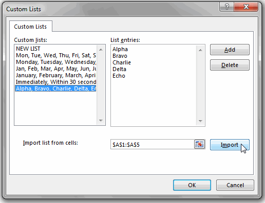
- Clicking on ‘Import list from cells:’ (pictured) will create a recognised list.
- Alternatively, you can simply select ‘NEW LIST’ from the ‘Custom lists:’ block and then just type in the list entries into, er, ‘List entries:’ and then press ‘Add’.
- Lists may be removed by highlighting the redundant list in the left hand pane and clicking the ‘Delete’ button.

