Comparing Lists Simply

Liam Bastick highlights some of the ways to avoid the need to use macros in financial modelling / Excel spreadsheeting.  This article highlights how to compare (multiple) lists without macros or even complicated formulaic logic (well, sort of…).

A Useful Functionality

I am not a great fan of PivotTables, truth be known.  Their results are sometimes a little too “black box” for my liking and many users forget to refresh them when data has been updated.  Power Pivot supersedes much of their functionality, but they are useful upon occasion. 

And this is one such occasion.

Let’s imagine you have a workbook with multiple lists contained in different sections or even worksheets.  For my example, I am going to assume we are comparing lists of colours, but these data points could just as simply be account codes, business units, employee names, etc.

Which colours are in all five lists?  Are there any duplicates within a list?  Do some colour descriptions have additional blanks after the end of the visible characters which may cause problems for LOOKUP or SUMIF operations?

How would you go about analysing these lists?  Many analysts would use conditional formatting to highlight duplicates or use functions such as VLOOKUP, COUNTIF and SUMIF to identify and reconcile list elements.  Others would resort to VBA and create a report that lists the number of occurrences of each item in list and in combination.

There’s a simpler way: PivotTables.

However, before going into full solution mode, I am going to make these lists more versatile by converting them into Excel Tables.

Turning Tables

With the release of Excel 2007, the Table functionality was introduced, superseding Excel 2003's ‘List’ feature, in effect adding functionality.  This has nothing at all to do with Data Tables.

Creating a Table in Excel 2007 and later versions is straightforward, and simply requires the user to select the data to be used in the Table.  You do not even need to select the whole range: Excel will prompt for the whole Table even if only one cell is selected (PivotTable creation works similarly).

Next, from the Ribbon, in the ‘Styles’ group of the ‘Home’ tab, click on the button that says ‘Format as Table’:

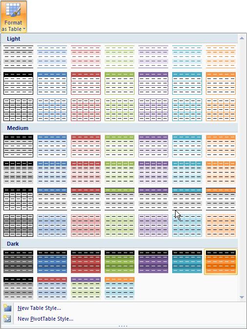
After clicking this button, Excel shows a new user interface element called a gallery, with a number of formatting choices for your Table, as displayed above.  New styles may be created by selecting ‘New Table Style…’ if required.

After one of the formats has been chosen, Excel will prompt the user regarding which cells are to be converted to a Table:

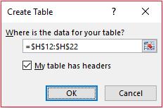
If the Table contains a heading row, ensure that the ‘My table has headers’ checkbox is checked.  Click ‘OK’ to convert the range to a Table.  The keyboard shortcut CTRL + T will have the same effect without allowing you to choose the formatting.

Tables have various useful functionalities, one such being the filtering which was done in lists in Excel 2003 and earlier versions.  For example, provided the Table has a header row, it will always have in-built filter and sorting, which can be readily accessed from this top row.

A Table will automatically resize to accommodate additional rows and / or columns, provided that data is entered in a cell immediately after the last column or row.  It is this feature that is particularly useful when dealing with our lists problem.

Back to the Example

I have turned my lists into Tables.  For example, the first list,

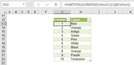
This Table has been given the unimaginative name First_Table (it’s always a good idea to name your Tables) and had a counter added for reasons that will become apparent shortly.

As an aside, for those that don’t work with Tables often, or do but encounter the following issue, do note how I have created the counter here.  I have used the formula

rather than =SUM($G$13:$G13) (say).  The SUBTOTAL(3,…) function works like COUNTA, i.e. it counts non-blank cells within the range – but with the added benefit of counting only the cells visible after filtering.  The second argument requires a little more explaining though.
The problem with =SUM($G$13:$G13) is that if the table is expanded with rows added at the bottom of the Table, the formula does not update correctly in the bottom rows.  Whilst it works correctly in the final row, rows directly above it have the same formula which leads to incorrect running totals, counters, etc.

The reference INDEX([Colour],1):[@Colour] circumvents this issue.  [Colour] is the entire field ‘Colour’ and INDEX([Colour],1) is therefore the first item in the field which is held constant (similar to $G$13).  [@Colour] gives the contents of the field ‘Colour’ on the row that the formula is in, so essentially INDEX([Colour],1):[@Colour] is $G$13:$G13 – it’s just that it works for some reason!

The second list is also turned into a Table with a counter:

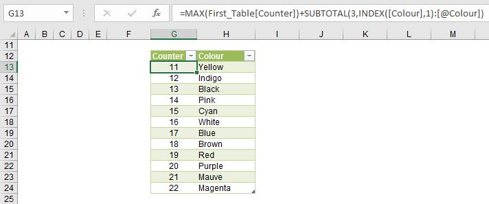
Here, note that the formula is slightly different:

This formula adds MAX(First_Table[Counter]) to the counter so that the counter continues from where the First_Table counter ends.  This logic is then applied to similar formulae in the Tables created for the next three lists too.

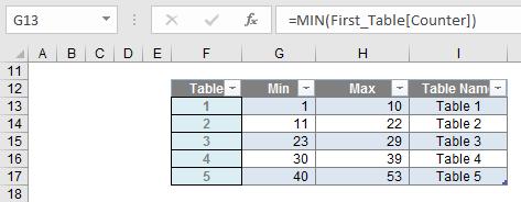
Next, a Table_Summary is created.  This summarises each Table’s name and the first and last counter in each using MIN and MAX functions respectively:

A dynamic, combined list can now be constructed using LOOKUP formulae.  This may seem convoluted (for those who know and have access to Power Query / Get & Transform [Excel 2016] with Power Pivot, a similar result can be achieved simply with appending Tables), but it will make your life simpler:

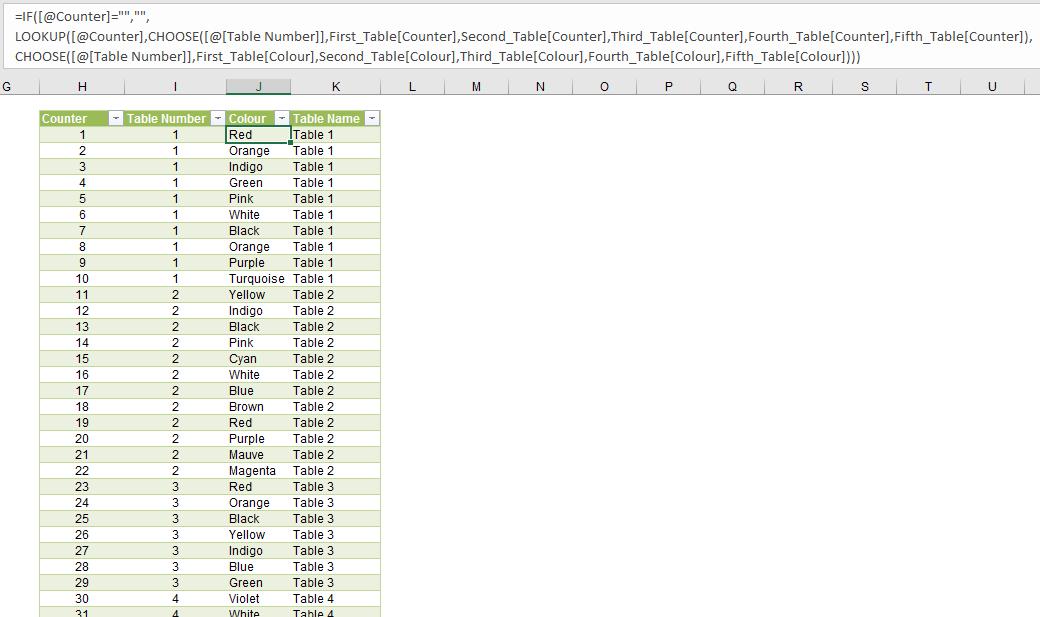
Upon first glance, the formula in the ‘Colour’ column looks horrible:

Once you get your head around it, it’s not quite so bad.  The LOOKUP seeks out the counter in the correct Table’s ‘Counter’ column and returns the corresponding colour from that Table.  The IF statement is applied simply to return a blank if the consolidated Table has more rows than there are in total in the individual Tables.

Once this has been generated, this can be used as the source for a standard Excel PivotTable (ALT + N + V, ALT + D + P or else highlight the entire Table and click on the Quick Analysis button in the bottom right-hand corner of the selection in Excel 2013 onwards), viz.

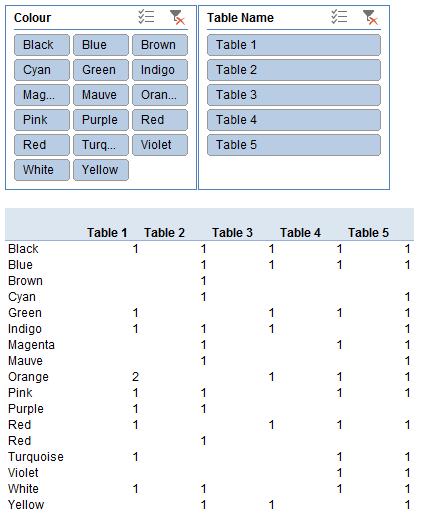
Now look how user-friendly this is!  It has slicers added to drill down on comparisons between the lists or even for each colour – and you can add items to all five lists or even add more lists (as long as you remember to refresh the PivotTable first).  Did you catch one ‘Red’ has an extra space or that there were two occurrences of ‘Orange’ in the first list?  Me neither.

I have taken the liberty of adding slicers to make the experience more user-friendly.  Feel free to download the associated Excel file here.  The numbers in the PivotTable could be formatted differently (e.g. conditional formatting) to make the summary even easier to follow.  How hard would this have been to do with formulae..?

No macros, no complex output formulae.  Simple to use.  Result.