Conditional Custom Number Formatting

Liam has provided financial modelling services and training to clients for more than two decades.  A director and professional mathematician, he has worked in numerous countries with many internationally recognised clients, providing and reviewing strategic and operational models for various key business assignments.

Given that one of the primary purposes of a spreadsheet is to present numerical data, it is important how such information is presented.  Cells may be individually formatted, using CTRL + 1 or ALT + H + O + E in all current PC versions of Excel.

Formatting only changes the appearance, not the underlying value, of a cell.  For example, if cells A1 and B1 had the number ‘1.4’ typed in but were formatted to zero decimal places, then if cell C1 = A1 + B1, you would truly have 1 + 1 = 3 (well, 1.4 + 1.4 = 2.8 anyway).

Excel has many built-in number formats that are relatively easy to understand, e.g. Currency, Date, Percentage.  The default format is ‘General’ where Excel will endeavour to provide the most appropriate format for the contents.  For example, typing ‘3 3/4’ into a cell will result in Excel selecting a mixed format.

But what do you do if you can’t find an appropriate format?

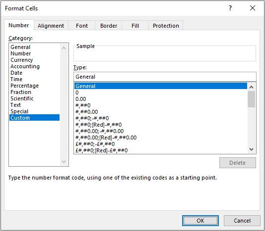
Selecting the ‘Custom’ category activates the ‘Type:’ input box and allows between 200 and 250 custom number formats in a particular workbook, depending upon the language version of Excel that has been installed.

The ‘Type’ input box allows up to four aspects of formatting to be specified in a cell.  These aspects are referred to as sections and are separated by a semi-colon (;).  To ascertain what is contained in each section depends on the total number of sections used, viz.

To the uninitiated, coding custom number formats may appear incomprehensible.  However, understanding the following soon puts things into perspective:

The above is not a comprehensive list, but it’s got most of the usual suspects.

To demonstrate, here’s a comprehensive example:

This format has all four sections, so the first section, [Blue]$* _(#,##0.0,_0_), specifies the formatting for positive numbers.  In this case, positive numbers will be formatted blue and be preceded with a $ sign.  Note the use of the asterisk followed by a space: this means that the cell width will be ‘padded out’ with spaces so that the dollar sign will be pushed to the very left of the cell and the number formatting will be to the very right.  _( is not necessary, strictly speaking, but ensures there is space made for an open bracket, even though there is no such character shown.  #,##0.0, ensures positive numbers contain thousand separators (where needed) and displays the number to the nearest 0.1 of a thousand.  Two commas at the end would have the number displayed to the nearest 0.1 of a million, and so on.  Finally, the _0_) requires Excel to maintain enough space at the right end of a cell for a digit (not necessarily zero and a close bracket).  It should be noted that a separate underscore is required for each character that is to be allowed for.

The second section, [Red]$* (#,##0.00,), specifies the formatting for negative numbers.  It is similar to the first section, but colors the number red, reports numbers to 0.01 of a thousand and encloses it in brackets.

The third section, [Color 7]\-_._0_0_), specifies the formatting for zero values.  This colors zero values “Color 7” which is a delightful pink in Excel’s standard color palette.  I am a great believer in using a dash, generated by using \- here, to denote zero as it distinguishes a zero value from something that is approximately zero, which can be useful for error checking, etc.  The final four underscored characters, _._0_0_), ensure that the dash will line up with the units value of a positive or negative value.

Finally, the fourth section, [Cyan]@*."is text", defines how text is to be formatted.  If omitted, text is simply formatted ‘generally’, but here it will be colored cyan.  The @ symbol specifies the relative location of the text within the cell (left-hand side of the cell), the *. will ‘fill’ the cell with period characters and "is text" will add these words to the end of the text, right-aligned (note no ‘&’ concatenation is required since these words appear in the formatting only).

There’s another way it can be used though:

Above, I mentioned what the four sections ‘generally’ mean.  This example highlights that this is not always the case.  Custom number formats allow up to two conditions to be specified.  This is because only four sections are allowed for custom number formatting and two are reserved.  The fourth section always specifies text formatting and one other section is required to detail how ‘everything else’ (numerically) will be formatted. 

The conditions are included in square brackets such that if the condition is true, the following formatting will be applied.

In this example, there are only three sections, so text will be formatted ‘generally’.  The first section, [>=1000000]#,##0,,"M", will format all numbers greater than or equal to a million to the nearest million and add an “M” to the end of the number. 

The second section will only be considered if the first condition is not true, so the order of the two ‘conditional formats’ needs to be thought through.  Here, the second section, [>=1000]#,##0,"K", will format all numbers greater than or equal to a thousand (but necessarily less than a million) to the nearest thousand and add a “K” to the end of the number.

The third and final section, 0, will format all other numbers (every value less than 1,000) to the nearest integer without thousands separator(s).  Pretty cool, eh?

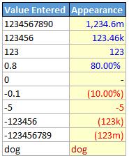
So far so good, but this could have all been gleaned elsewhere.  Let’s turn this idea up to 11.  Imagine you wanted to format a cell so that the following values would appear as follows:

The issue here is how to create the correct formatting without using VBA code or Excel formulae in ONE cell so that if any of the above values in the left-hand column are entered into that cell they will appear as they are displayed in the right-hand column.

There’s too many examples to use custom number formatting here – I want things in positive and negative millions (formatted differently), positive and negative thousands (formatted differently), positive and negative numbers in absolute terms below 1,000, positive and negative percentages (formatted differently), zeroes and text.  I’m becoming exhausted just typing this – never mind figuring out how to do it!

Conditional Formatting

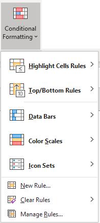
Conditional formatting was completely revamped and reinvented with the introduction of Excel 2007.  Located in the ‘Styles’ group of the ‘Home’ tab, it’s an ‘OD’ feature allowing you to ‘OD’ on number formats using the keyboard shortcut ALT + O + D:

I can use ‘New Rule…’ to exploit a loophole in the restrictive number of conditions custom number formatting appears to allow.

Using custom number formatting and conditional formatting combined the requirement is fairly straightforward.  My suggested solution would be:

• Construct the underlying number formatting first.  Personally, I would use custom number formatting so that all positive and negative numbers appeared as percentages, zero as a hyphen and text as displayed above:
  [Blue]_(#,##0.00%_);[Red](#,##0.00%);-;@
• Next, I would apply conditional formatting number formatting where the cell value is greater than one so that numbers greater than a million could be displayed to the nearest 0.1m, numbers less than a million but greater than or equal to 1,000 could be displayed to the nearest 0.00k and numbers lower than 1,000 (but necessarily greater than one) could be displayed as integers:
  [Blue][>=1000000]#,##0.0,,"m";[Blue][>=1000]#,##0.00,"k";[Blue]0
• Finally, I would apply a second set of conditional formatting where the cell value is less than -1 as required:
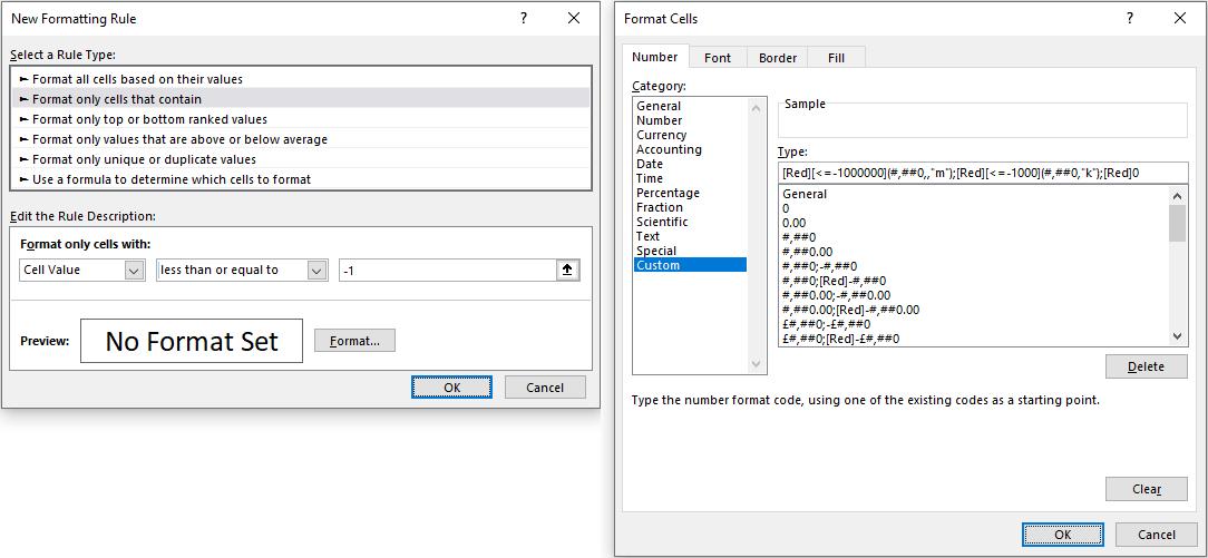
  [Red][<=-1000000](#,##0,,"m");[Red][<=-1000](#,##0,"k");[Red]0

Here’s an illustration of that final formatting:

In this above illustration, I have selected conditional formatting to occur if the value in the cell is less than -1.  Pressing the ‘Format…’ button then allows the user to select how the number formatting might appear.

Since many, many conditional formats may be applied to one cell in Excel, you can soon apply significantly more than four formats to any cell(s) in Excel.  As is often the case with Excel, when all else fails – cheat!

Word to the Wise

Although I have explained you can circumvent the apparent limitations in number formatting using conditional formatting, applying too many unnecessary conditional formats can cause Excel to misbehave with cells not updating as intended and other cells (not formatted) changing as well.

Further, using lots of custom number formats in a single workbook uses considerable memory and can slow down the calculation time of an Excel file unnecessarily.  Many of these formats are created accidentally.  Each time a custom number format is edited, it will generate an additional listing for Custom Category Types.  Any custom formats created inadvertently in this manner (that are not being used in the file) should be deleted; good housekeeping is essential.