Controlling Your Inputs
This article considers one of Excel’s useful input functionalities: data validation. By Liam Bastick, Director with SumProduct Pty Ltd.
Query
Is there any way in Excel I can control what end users can type into a cell?
Advice
There are several ways this can be done, but arguably the simplest is data validation. I must admit that this is one of Excel’s functionalities I am guilty of assuming everyone knows. However, this isn’t the case, but similar to Formats & Styles once you use this functionality and understand what it can do for you, you never go back.
To access data validation, from any cell in Excel:
Excel 2003 and earlier
- From the drop down menus, go to Data -> Validation… (ALT + D + L)
Excel 2007 and later
- On the Data tab of the Ribbon, go to the Data Tools group and click the Data Validation icon (ALT + A + V + V)
- ALT + D + L still works
This brings up the following dialog box:
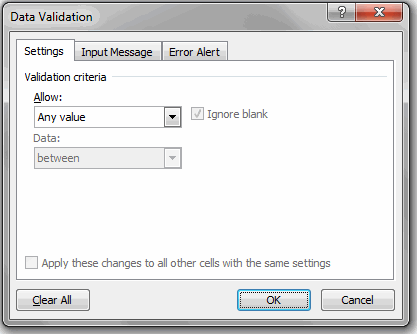
The default setting for all cells in Excel is to allow any value (pictured). This can be changed by changing the selection in the ‘Allow’ drop down box. It may be modified to any of the following:
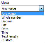
Most of these criteria do exactly what they say on the tin: by choosing ‘Decimal’, the input must be a number, whereas ‘Whole Number’ allows for integers only. However, making a selection from the ‘Allow’ drop down box is only the first part of the data validation process.
Once a selection has been made (for example, I will use ‘Whole Number’), the dialog box will change appearance, viz.
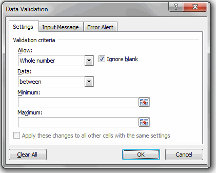
The ‘Ignore blank’ check box is no longer greyed out. This allows blank cells to be ‘valid’ regardless of the criteria selected. The remainder of the dialog box is governed by the ‘Data’ drop down box. There are various selections that may be made:
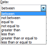
Depending upon the choice made, the box will prompt for values (e.g. Minimum and Maximum in the illustration above) which can be typed in, or else the values can refer to cell references directly or indirectly via range names.
One the choices have been made, you might wish to utilise the other two tabs of the Data Validation dialog box.
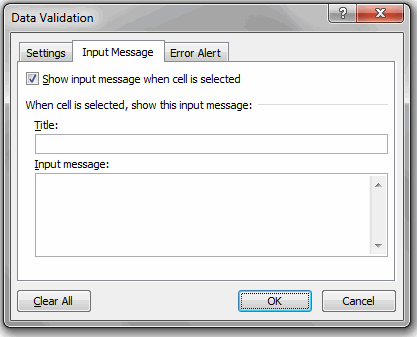
With the ‘Show input message when cell is selected’ checked, if the end user selects the data validated, cell the message typed in here will appear. This can make data inputs in a model much simpler as end users are ‘spoon fed’ with a pop-up box detailing what to do. In the example below, the ‘Input Restrictions’ comment only appears when the cell is selected:
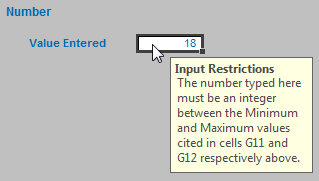
The third tab selects what to do if invalid data is entered in the cell:
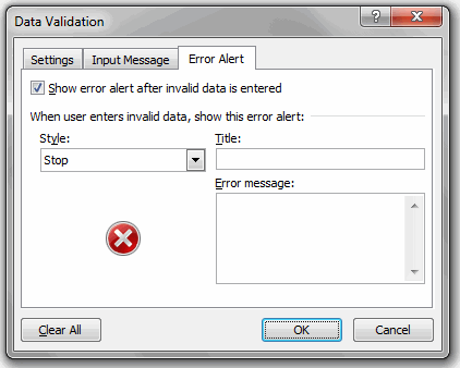
This alerts the end user when an invalid entry has been made (e.g. typing “dog” when a number is expected) – as long as the ‘Show error alert after invalid data is entered’ check box is ticked.
There are three styles available:
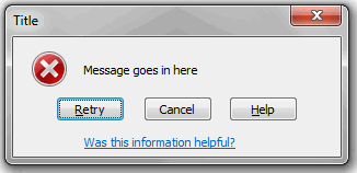
Stop
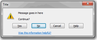
Warning
Information
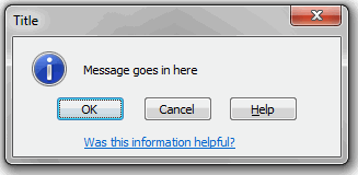
The three styles provide differing treatment of invalid data:
- Stop – the value will not be accepted and the end user will be prompted to retry;
- Warning – the end user will be warned that the data is invalid, but be asked whether it is OK to continue;
- Information – the end user will be advised that the data is invalid but that the data has been accepted.
If the ‘Show error alert after invalid data is entered’ check box is not ticked, no prompt will occur and invalid data will be accepted in the cell without any warning.
Other Types of Data Validation
Whole Number, Decimal, Date, Time and Text Length are all relatively straightforward, albeit very similar in nature. This leaves just two remaining categories to consider.
List
This functionality allows the end user to select from a list.
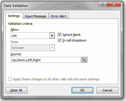
With ‘List’ selected, the dialog box prompts for a source for the list. In the illustration, the entries have been typed in, separated by a comma. However, the data can use cell references which are in a column – or a row – as long as the cells are on the same worksheet. This can be limiting and a viable workaround is to name a row or column of data (see Range Names for more details) and then use the range name here.
For lists, I strongly recommend using the ‘In-cell dropdown’ which provides a dropdown list of valid entries once the cell has been selected.
Custom
As you become more experienced, you may find the functionality limiting. This is where the final ‘Allow’ category comes in useful, as you design your own data validation. Examples are included in the attached Excel file.
Word to the Wise…
Data validation will not solve all of your data entry problems. If data has already been entered into a cell and data validation is applied retrospectively such that the contents of the cell would be deemed invalid, no warning will ensue. Similarly, if the contents of a list are altered, any cells that selected the changed value will not update automatically.
To counter these issues, invalid data may be identified on a worksheet as follows:
Excel 2003 and earlier
- From the drop down menus, go to Tools -> Formula Auditing -> Show Formula Auditing Toolbar (ALT + T + U + S)
- From the toolbar, click circle invalid data

Excel 2007 and later
- On the Data tab of the Ribbon, go to the Data Tools group and click the drop down menu next to the Data Validation icon
- Select ‘Circle Invalid Data’ (ALT + A + V + I)
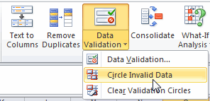
This will circle all invalid data on the worksheet.
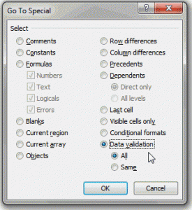
One other issue is locating cells that have been data validated in the first place (i.e. no longer allow ‘any value’). The simplest way to do this is through the ‘Go to’ dialog box (F5), click on the ‘Special…’ button and then select ‘Data Validation’ (either all data validated cells or those validated similarly to the cell presently selected):
Select ‘Special…’ on the Go To Dialog Box
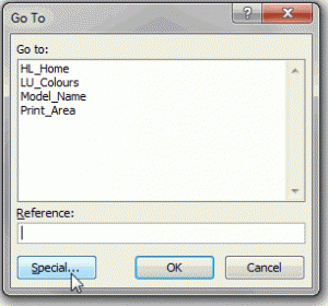
Choose Data Validation
