Entering the Import / Export Business

Liam Bastick highlights some of the common issues and scenarios in financial modelling / Excel spreadsheeting.  This time we look at tips for linking data between workbooks.

File Linking

Before I start, I’d like to emphasis try not to link workbooks, where possible.  Managing links and detecting the dreaded “phantom links” (i.e. links which are unintended) may become a major preoccupation if proper care is not taken.  Nonetheless, linking workbooks is sometimes required.  Legitimate reasons may include:

• Not sharing confidential data (don’t make the mistake of trying to “hide” data – there are countless stories the stuff of legend where businesses have been embarrassed attempting to adopt this approach)
• Files are too large to open in a 32-bit environment
• Files are too large to email.

Standard industry practice to link two workbooks together tends to conform to the “URM” approach, viz.

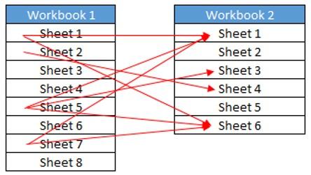
That’s right, meet “URM”: the Utterly Random Method.  This technique is inadvisable and dangerous.  It makes it difficult for end users to identify external links or not be able to differentiate between intended and accidental links.  In fact, if links go both ways and only one workbook is open, circular references may be created and worse, be disguised.

If you do have to link workbooks, consider the following approach instead:

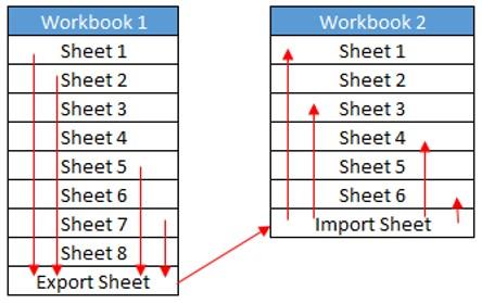
This approach is much more uniform:

• Identify all cells that need to be exported (i.e. linked to another workbook)
• Link these cells all to a dedicated ‘Export’ worksheet
• Create a mirror image, dedicated ‘Import’ worksheet in the destination workbook
• Refer to these imported cells in the other sheets.

This way, it is easy to trace and locate all external references.  Should you have multiple worksheets to link to, simply create separate import / export pairs for each link (do not put them all in the same worksheet as this will confuse end users).

Some commentators and “Best Practice” guidelines will recommend using a range name for either the source and / or destination cell(s) of the relationship link.  Personally, I am not a fan of this method.  I understand the main reason for this.  Using range names will address the issue of inserting or deleting rows and / or columns whilst the linked file is closed; standard cell referencing will not. 

It is true range names will overcome this issue.  However, the problem is many users cannot readily locate range names and problems may arise with multiple workbooks open with similar or the same range names, especially if you have multiple copies of a particular worksheet.  This can, in fact, lead in a worst-case scenario to file corruption.

So what should you do instead?

It’s very simple, if not ideal.  After creating import / export sheets in the way explained above, either hide or protect these said sheets.  Their sole purpose is for linking to other workbooks so there is no need to revise the worksheet structure after they have been agreed and created.  Yes, you might insert rows or delete columns within an internal worksheet of one workbook whilst the other associated files are closed – but the links will remain intact to the relevant import or export sheet.  Simple!

This just leaves one question: how do you create a “mirror image” worksheet?  Here’s an example of how easy it is to do this…

Example

The first thing to do is clearly identify the data that needs to be linked to another workbook (i.e. the data to be exported data).  Create an export worksheet and link all the data in:

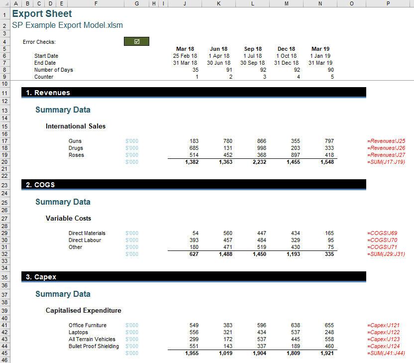
(The formulae in the red cells are displayed to show where the data may have come from and these cells do not form part of what should be exported.)

After creating a blank sheet in the destination workbook, it’s now time to create the “mirror image” import sheet.  To do this, highlight the entire ‘Export Sheet’ by selecting the grey corner cell in the row / column headers:

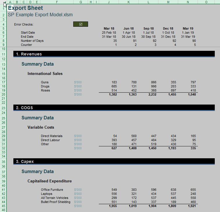
Now copy this sheet (CTRL + C).  Select cell A1 in the destination worksheet and paste special as values (ALT + E + S + V + ENTER):

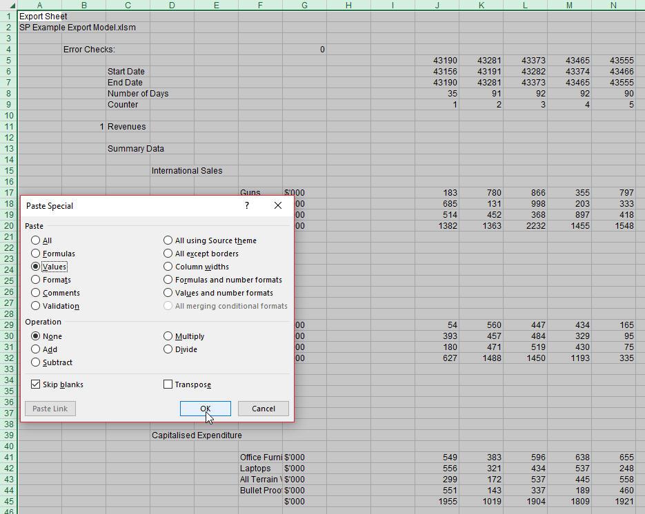
Immediately afterwards, copy and paste special as formats (ALT + E + S + T + ENTER) too:

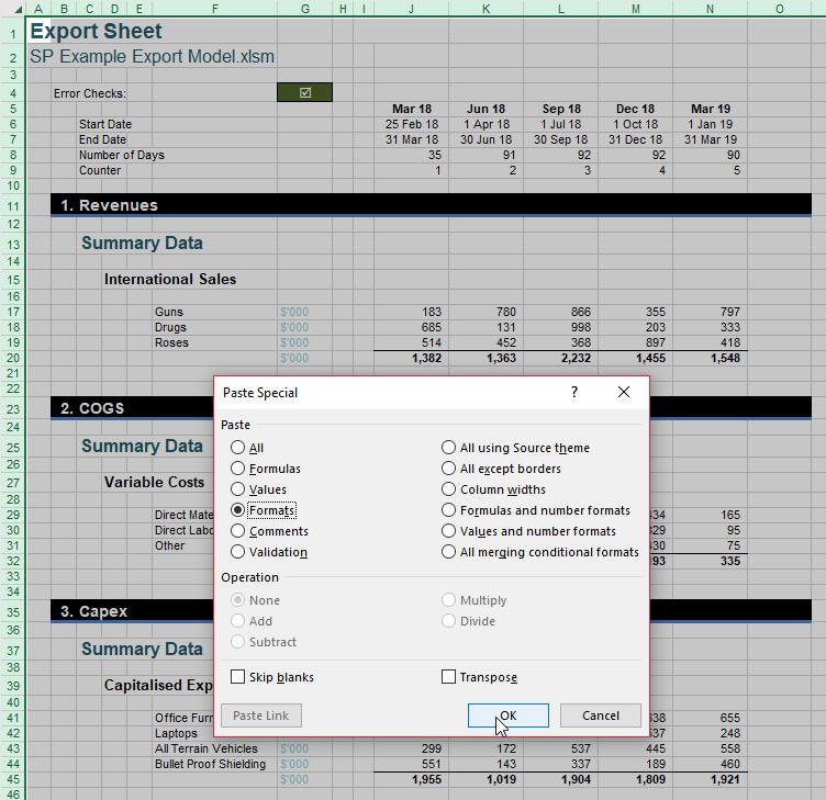
Note that if you had gridlines turned off in the source worksheet, this setting will not be replicated in the destination sheet.  These may be turned off easily though by going to the ‘View’ tab in the Ribbon and unchecking ‘Gridlines’ in the ‘Show’ group (ALT + W + VG).

You must paste as values before you format – this order is important.  This is because if you have any merged cells, formulae will not copy across after merging.

Once these actions have been taken, you should have a worksheet that looks like this:

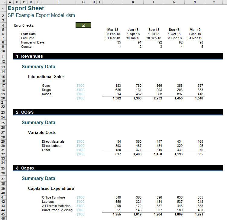
It looks like the original, but with all of the data, labels and dates hard coded.  This is intentional – we’re not finished yet!

Do you see the sheet title in cell A1 is incorrect?  Well, guess what, I am not going to fix it yet.  In fact, I am going to “reinforce” this error.  I am going to link cell A1 in the import sheet back to cell A1 of the source export sheet.  Given the other workbook must be open by definition, the formula in cell A1 will look something like this:

Note that all cells linked to other workbooks are made absolute (i.e. use dollar “$” signs) by default.  I need to remove this pair of dollar signs, so I have relative referencing:

This will mean as we copy this formula into other cells in the import sheet we will always be linking back to the corresponding cell (e.g. cell B17 will link to B17, cell AA686 will link to AA686 and so on).  This is what we want. 

Once this change has been made, copy this formula (CTRL + C) into cell A1 of the import sheet.  Now, I need to select where I am pasting this cell.  I do not want to paste it into all cells in this sheet, just the non-blank ones.  To do this, I load the ‘Go To’ dialog box (function key F5 or the keyboard shortcut CTRL + G):

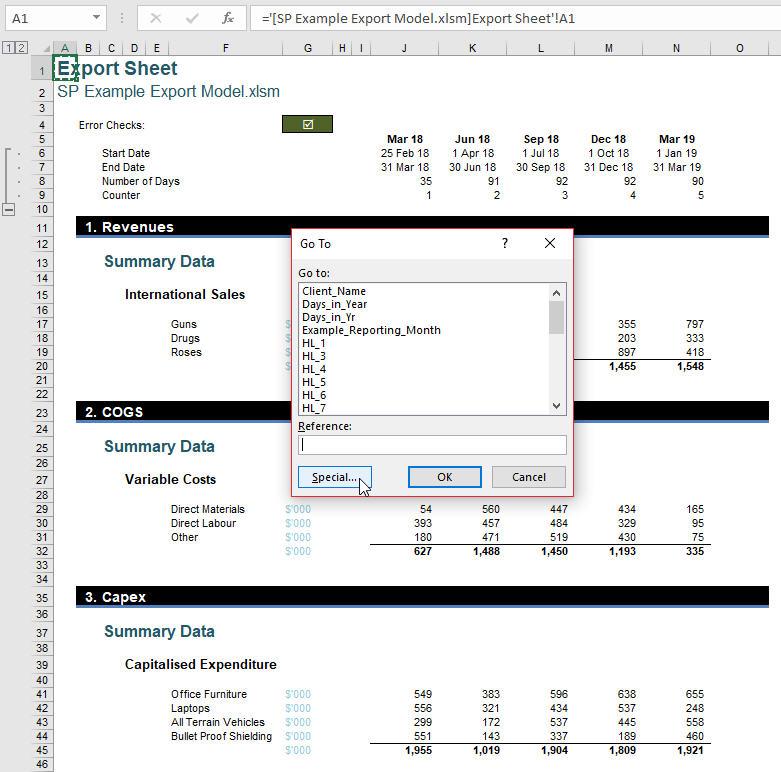
Next, I click on the ‘Special…’ button in the bottom left-hand corner:

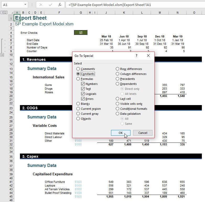
I select the ‘Constants’ radio button and ensure the ‘Numbers’, ‘Text’, ‘Logicals’ and ‘Errors’ checkboxes are all checked as displayed (above).  This means every non-blank cell will now be selected, viz.

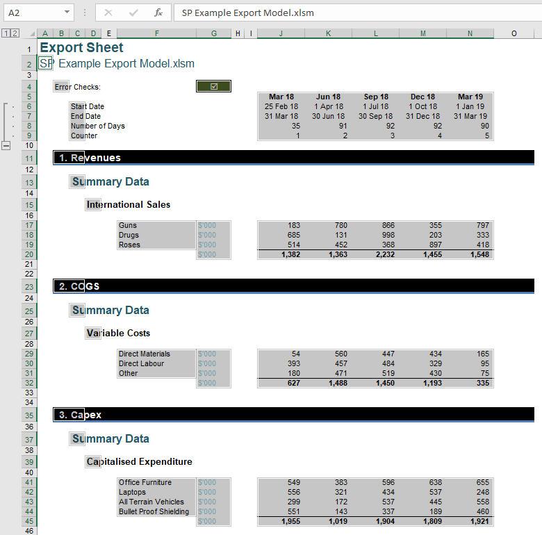
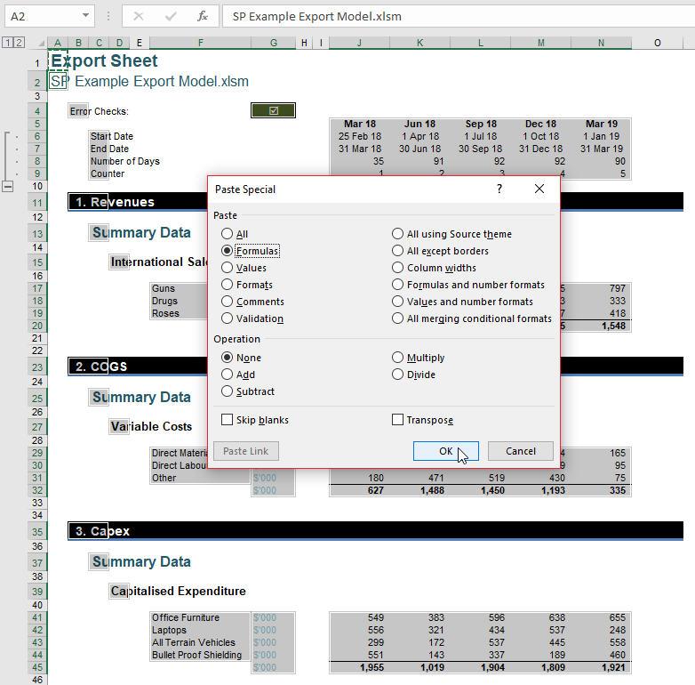
Note cell A1 is not selected (it’s a formula!).  Now, I just paste special as formulas (sic) (ALT + E + S + F + ENTER):

I now have an import sheet where all non-blank cells link back to the export worksheet:

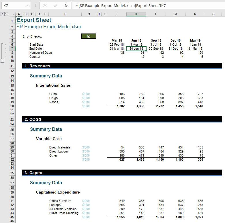
All I have to do now is correct cells A1 and A2, which need to say “Import Sheet” and cite the filename of the destination workbook respectively.

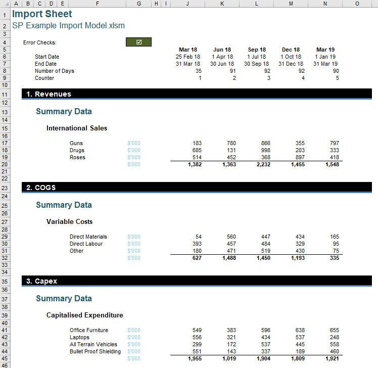
If you have more than one link, this process will need to be repeated for each import / export pair.  Don’t try and have just one import or export worksheet – it gets too confusing. 

Word to the Wise

This may seem like an over-the-top solution to a common problem, but with practice, this process takes only seconds to perform and can save hours later as you go seeking those pesky links when you have forgotten where they might be!