Go Poisson

Cecile Nguyen likes fishing for answers.  This article looks at calculating the inverse of a Poisson distribution for scenario modelling but with the caveat this is a simple, pragmatic approach for non-academics.

Continuing on from Simulation Stimulation, let us look at another way to model scenarios.

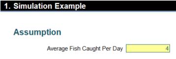
Let us look at modelling independent events that occur at a known and constant rate.  Let us say I go fishing.  Over long observation, I notice that I net four fish a day. The fishes are presumed independent from each other, i.e. a fish deciding to be caught has no bearing on the decision of another to bite.

Let’s look at the limiting factors in modelling this:

• Sometimes catching a fish might not happen, but I would never receive -2 fish on any given day
• Neither would I get portions of fish – it is all or nothing
• A large number of fish might get caught, but with small likelihood - I could theoretically amass 5,000 fish in a day though it is highly unlikely
• The events cannot occur simultaneously, there is only one fish on the line
• The expected average number is known over a certain time period.

Now why is the binomial situation inappropriate in this case?  The binomial distribution counts the number of occurrences in a set amount of trials whereas in this case there may be infinite events.

Let’s use ? to denote the mean number of events.  Returning to the n , p of the Binomial distribution, this would more closely model an infinite amount of trials i.e. n ? ? and the probability is decreasing p ? 0 in such a way that n p ? ? .This is known as a Poisson distribution and the mathematical proof can be viewed here.

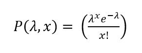
Thus, the likelihood of x events happening to a Poisson distribution can be calculated according to the formula:

where:

• ? = mean
• x = number of events modeeling subject to x = 0, 1, 2, ... 

Excel has two functions that can calculate it:

• POISSON(x, mean, cumulative).  When the last argument (cumulative) is set to TRUE, POISSON returns the cumulative probability that the observed value of a Poisson random variable with specified mean will be less than or equal to x.  If cumulative is set to FALSE (or 0, interpreted as FALSE), POISSON returns the calculated probability as per the formula above
• POISSON.DIST(x, mean, cumulative).  As above, but note that since Excel 2007, Microsoft has updated many of its statistical functions.  This more accurate function supersedes the POISSON function which remains for backward compatibility – for the time being at least.  If you are new to both of these functions, I would suggest using this variant as Microsoft has advised it may not support the former function in future versions of Excel.

The attached Excel file provides an example of the Excel function can be used in practice:

Simulations Analysis in Excel

Similar to Simulation Stimulation, we’d like to use the simulations method to model the number of fish caught in a day.  However, unlike NORM.INV, Excel does not provide a Poisson Inverse function which means that we had to write our own. 

Let’s look at the logic of the Poisson function and create our own User-Defined Function in VBA (which we have called PoissonInverse):

• Check that the probability we want to check is within the bounds and return 0 if the probability is 0
• Because of the relationship between Binomial and the Poisson distribution for sufficiently high number of trials, n p ? ?, we can use the Binomial inverse to estimate x.  We can generate the “number of trials” by using n = ? / p . Thus, we can use the following function

BINOM.INV(number of trials, mean / number of trials, probability)

• With our estimate for x, using POISSON.DIST to retrieve the cumulative value at  and then loop forward or backwards accordingly to determine that this is the correct value that the minimum cumulative value is greater than the probability supplied.

The workbook has the macro inside but the macro code in text format is attached here for the security concious.

We can get Excel to pick a random number between 0 and 1 using the  function.  There is no situation a value of 1 is permissible but luckily the RAND() only calculates on the [0,1) interval, i.e. the number must be greater than or equal to zero but strictly less than one.  For a given mean, this will generate a particular outcome appropriate to the probability distribution specified, which can then be used in the model as in the following illustration:

We want to model how many fish we catch over a 1,000 day period with an average of four fish per day.  As per the above points, we believe this to be Poisson distributed.  Using the RAND() function to generate probabilities, using our newly created PoissonInverse function we can model how many fish are caught in a given day and then chart the frequency.

With that, we can see that our average is calculating very close to average the model is supplied and the frequency looks quite pretty: