How Much Do I Need?

As lockdowns became more and more the norm and businesses ramped back accordingly, the recent global environment brought physical, psychological and financial strains more to the fore than ever before.  I wish readers all the best in these troubled times. 

I am not the sort of professional that can assist with the first two pressures, but I can help you to be more informed about the third.  And that’s half the battle.  When business slackens, you need to control your cash before it controls you.  Therefore, let me help you analyse your future cashflow requirements as follows.

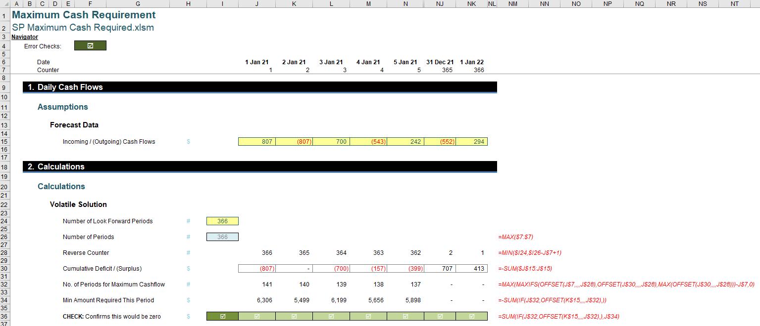
With the assistance of the attached Excel file, let’s imagine you run a business.  As cashflow reduces, the need for more accurate and granular forecasts becomes greater.  Therefore, you have forecast the following daily cash flow profile (in extract):

In my Excel file, these cash flows have been predicted for 366 days.

Presently, you know how much cash you have in reserve.  The question is, how much do you need to get you through these tough times?  The sooner you identify the amount and the shortfall (if any), the sooner you can make contingency plans, such as reducing costs, organising loans, etc.

For any particular start date, the answer appears simple.  All you need to do is keep a running total of the cashflows for each period, and calculate the minimum value.  For example:

Here, I have created a running total in row 17 using the simple cumulative summation

Then, I simply identify the minimum value in cell I19:

(N.B.  The minus sign in the formula is used to avoid confusion: negative shortfalls would confuse many.)

This shows the largest negative value will be $5,499 – and this is the amount that I need (now) to ensure there is never a shortfall. 

Wrong.

This is a common mistake made by businesses time and time again.  It is commonly held that replacing the first period’s value of $807 with $5,499 will prevent shortfalls.  This is incorrect:

With $5,499 used in the first period, there is still a requirement to fund $807.  $807?  Where have I seen that before? 

This amount was the amount originally in the first period.  That makes sense.  The shortfall already included the amount in the first period.  Our calculation simply identifies the additional amount required.  This would be $5,499 + $807 = $6,306. 

This can be calculated as follows:

We almost had the calculation correct.  The running total needs to exclude the current period, and start from the next one and then be computed for all periods until the end of the forecast period.

This is all we need to do if we simply want to calculate the requirement for the first period.  But what if we want to “roll” our forecast and identify what we need on the 17 August (say) instead?  You could repeat this exercise and simply have a similar calculation on each row for each period, similar in appearance to a depreciation schedule.  That would require 366 rows and at least 67,161 formulae!

Surely there is a better way?  Yes there is – and stop calling me Shirley.

Let me add another complication too: it might be you only want to see what the maximum cash is needed for a certain number of days (e.g. circumstances may change, you may have other alternatives).  I will add in a selector, although I will set it originally to 366, so that we may compare with the original illustration (above). 

Then, consider the following calculations:

I can calculate the maximum cash required for any period using just five formulae (and even then, arguably you could condense some of these).

The first formula is situated in cell I24 (above).  This calculates how many periods have been forecast:

In general, you should never create a formula that refers to an entire row or column as they can use up resources, leading to lack of memory issues and poor calculation times.  However, this is a simple formula, and allows for additional periods to be added without issue.  It is only calculated once.  This is good practice: try never to calculate resource hungry expressions more than once.

The formula in row 26 then provides the reverse counter (like a countdown, but considering the stipulated look forward period).  For example, in cell J28, this is given by the formula

For a 366-period model with a 366-period look forward, this provides a countdown from 366 (first period) to one (1) (final period).

The third formula is the cumulative sum, e.g. in cell J30, it is given by

This formula is negated so that deficits are positive and surpluses are negative.  I find it easier for people to understand calculations where the results are positive. 

What we want to do now if from a given start position in row 28, we want to find the largest value, as this will represent the relative lower bound of the cashflow.  It is relative because this cumulative figure may include values that are past (sunk): it doesn’t matter, as the lowest value remaining will still be the lower bound, once adjusted.

This leads to an horrific formula, e.g. in cell J32, it is

Any questions?  Oh wait, I see there are. 

The MAX function is fairly straightforward (simply taking the maximum of its arguments), but the other two functions may require further clarification:

• the OFFSET(reference, rows, columns, [height], [width]) function has the height and width arguments in square brackets, as they may be omitted from the formula, as usually OFFSET deals with moving so many rows down and so many columns to the right of the reference. 

However, in this instance I am trying to define a range that, although only one row deep, is so many columns wide.  Therefore, aside from the reference and the width all of the other arguments may take their default values (zero [0], zero [0] and one [1] respectively).

Therefore, the expression OFFSET(J$7,,,,J$28) means take a range of cells in row 7, starting at J7 with a width of J28 columns.  Since J28 is 366 given the restrictions on look forward and the model duration, this means take the range of 366 cells in row 7, starting in column J, i.e. J7:NK7.  Similarly, OFFSET(J$30,,,,J$28) defines the range J30:NK30.  The beauty about the OFFSET function is that if the number of periods varies, this range will update automatically. 

This slowly contracting range is used rather than a fixed width that changes references (e.g. J30:NK30 in the first cell, K30:NL30 in the second, …) so that calculations are not any larger than they need to be.  An OFFSET formula is required as the width may vary based upon the Number of Look Forward Periods (cell I24) selected

• MAXIFS(max_range, criterion_range1, criterion1, [criterion_range2, criterion2,] ...) returns the maximum value among cells specified by a given set of conditions or criteria, where:
  
  • max_range is the actual range of cells in which the maximum is to be determined
  • criterion_range1 is the set of cells to evaluate with the criterion specified
  • criterion1 is the criterion in the form of a number, expression or text that defines which cells will be evaluated as a maximum
  • criterion_range2 (onwards) and criterion2 (onwards) are the additional ranges and their associated criteria.  126 range / criterion pairs may be specified.  All ranges must have the same dimensions otherwise the function returns an #VALUE! error.

The previous formula reduces to

MAXIFS(J$7:NK$7,J$30:NK$30,MAX(J$30:NK$30)) returns the counter in row 7 that identifies the largest cumulative deficit in row 30.  This occurs in period 142 for cell J32.  This means the formula is now

Since J$7 represents the first period (1), the resulting value is 141.  This means that the largest deficit is recorded when you sum the first 142 values in row 15 – but we subtract off the first period, so we do not repeat our previous mistake.

The formula in J34 then evaluates this summation:

(again, the negative sign to prevent confusion).  This formula is the same as

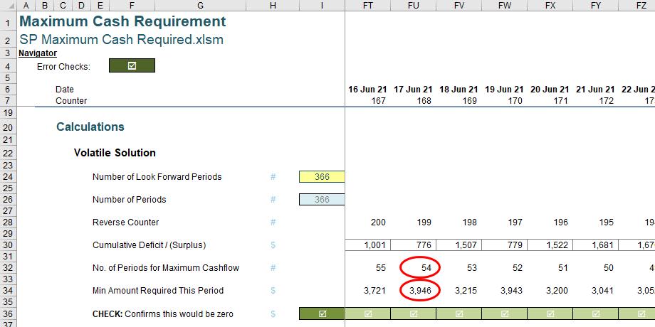
where K$15:EU$15 is the range of 141 cells across starting in cell K15.  This gives the same value we calculated earlier, i.e. $6,306.  However, unlike the previous method, the value in cell K34 ($5,499) shows me the value that should be in Period 2 to ensure no future shortfalls, and similarly the value in cell FU34 (period 168) advises me that on 17 June, I will require $3,946 in this period to avoid a cashflow shortfall based upon future projections from this point, with a minimum value of zero (nil) occurring 54 days later on 10 August (period 222).

The formula in row 36 (e.g. cell J36)

simply confirms that the value cited in row 34 is correct.

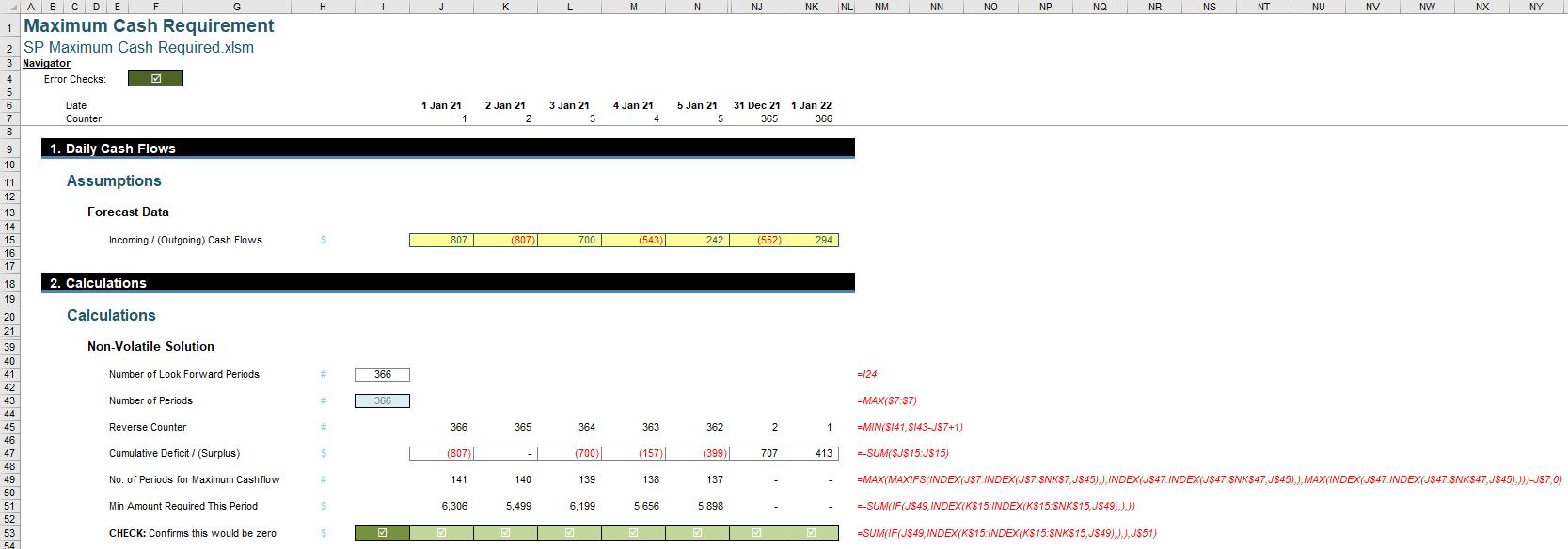
Regular readers that the OFFSET function both fools Excel’s auditing tools (e.g. Trace Dependents) and is volatile (i.e. a calculation that causes unnecessary recalculations of the formula in the cell where it resides every time Excel recalculates).  If calculation is speed / memory usage is important to you (e.g. where this calculation may form part of a very large Excel model), then you may wish to replace OFFSET with its non-volatile counterpart, INDEX:

I don’t explain this here; please refer to the attached Excel file for further details.

Word to the Wise

Some readers may view the above as a little basic.  It’s true; it is.  You can add greater complexity by:

• changing the number of days looking forward considering the time value of money (present values)
• allowing for surpluses to earn interest and deficits to incur interest payments and other fees
• including probability weightings to approximate the likelihood of the cash flows occurring
• incorporating direct and indirect tax cash flow consequences.

Whilst it is admittedly simplistic, it is greater analysis than many businesses do.  It is a start that you can build upon.  Hopefully, you find this useful and may put it to good use.