Keeping Up Appearances – Conditional Formatting

Advice

With Excel’s IF function, the contents of a cell can be modified depending upon (a) certain condition(s) being met (i.e. held to be TRUE).  However, the formatting or style of the cell cannot be changed in this manner.

Macros are not needed.

First introduced in Excel 97, conditional Formatting is an Excel feature that indeed allows you to apply formats to a cell or range of cells and have that formatting change depending on the value of the cell or the value of a corresponding formula.  This was one of the features that was given a major overhaul in Excel 2007.

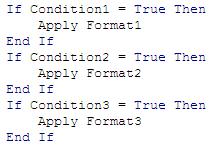
Accessed from the ‘Home’ tab (or ALT + O + D), conditional formatting formats the cell(s) selected depending upon whether a condition is TRUE.  In Excel 2003 and earlier versions, conditional formatting would work as follows:

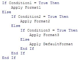
Essentially, as soon as Excel finds a condition that is held it formats accordingly and stops.  If none of the three conditions is met, the underlying format (i.e. the fourth format) is retained.

As explained above, conditional formatting was completely revamped and reinvented in Excel 2007.  Located in the ‘Styles’ group of the ‘Home’ tab, the conditional formatting feature has had a raft of new features added:

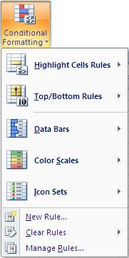
For instance, inspecting ‘Highlight Cells Rules’ is akin to many of the “Cell Value Is” functionalities of its predecessor, such as. Greater Than, Less Than, Between, Equal To, or even More Rules:

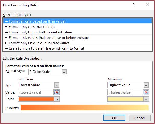
Other options are also available: Date Occurring and Duplicate Values.  All you have to do is highlight the list, select the option and colour scheme required.  Simple (no need to concoct hideous formulae such as =IF(COUNTIF($A:$A,$A1)>1,COUNTIF($A$1:$A1,$A1)>1) for locating duplicates, for example).

Users should not be fooled by the easy-to-use Top / Bottom Rules either.  Top 10 Items, Top 10%, Bottom 10 Items and Bottom 10% all highlight items that conform to these labels.  However, the ‘10’ can be changed to a number of the user’s choice.  Who could possibly live without the Bottom 37% Debtors Report for instance?

Above average and below average data can be highlighted also in one or two clicks and even graded shading of a cell as well.  For example, if cells A1:A10 had the values 10, 20, 30, …, 100 respectively, the cells could be filled in as follows:

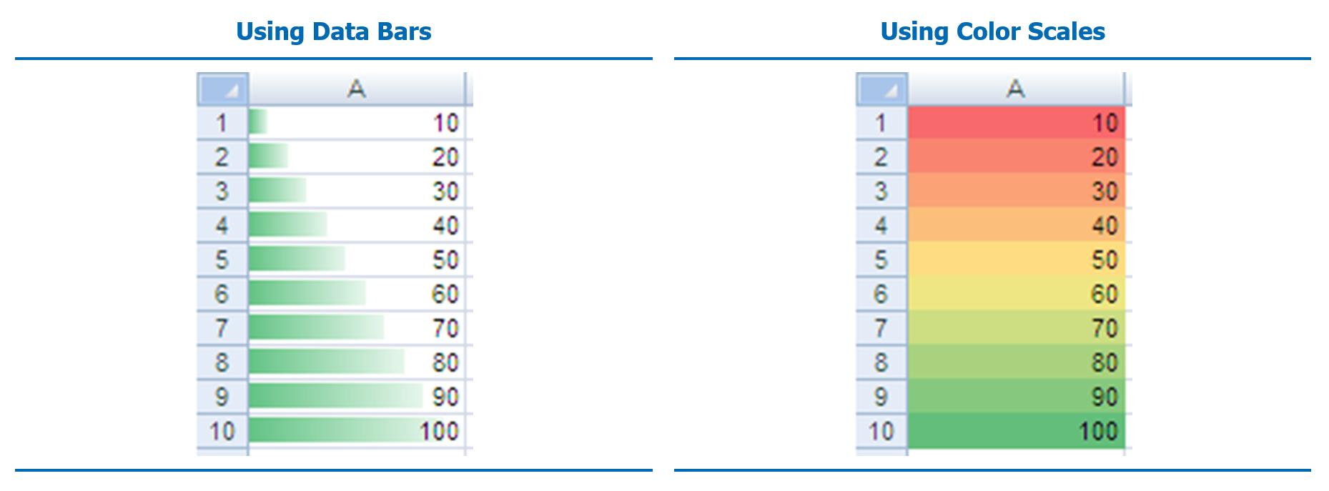
Clearly, looking at the Color Scales example, conditional formatting lends itself neatly to traffic light reporting.  This is compounded by Icon Sets that will stratify data into between three and five sections using various icons (such as the red, amber and green traffic lights).  Given that conditional formatting now permits cells to be sorted dependent upon their background colour (ALT + D + S, then choose ‘Cell Color’ in ‘Sort On’ field), you can make monthly reporting a colourful adventure!

Conditional formatting in Excel 2007 does differ logically from its predecessor. 

With Excel 2003 and earlier, as soon as Excel finds a condition that is held it formats accordingly and stops.  This can be performed for up three conditions.  These days, there is ‘no limit’ and testing does not have to stop (more than one format can be applied in a cell at a time), i.e.

To highlight this, consider the following data set before and after multiple conditional formatting:

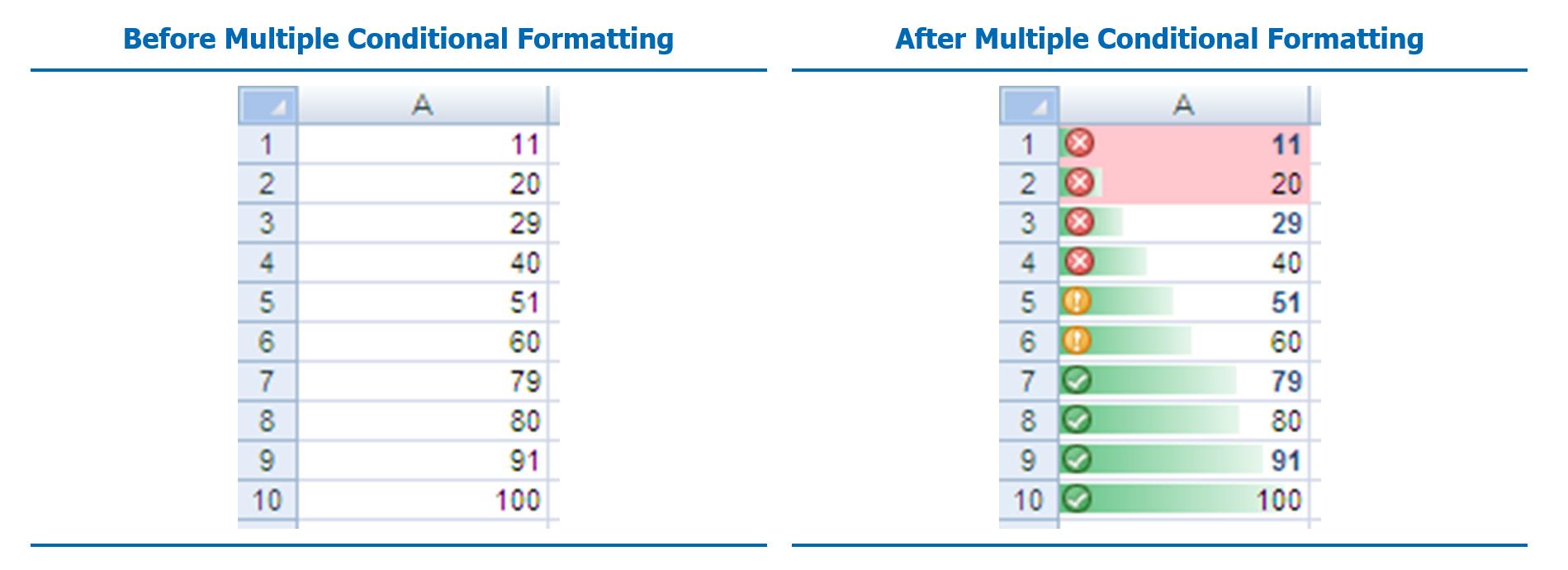
No less than four conditional formats have been applied, as can be seen by opening up the Conditional Formatting Rules Manager (ALT + O + D):

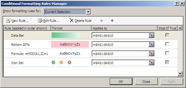
Using the blue up and down arrows can reorder the sequence and the sequence can be stopped if certain conditions are true (simply check the box in the fourth columns).  This gives conditional formatting significantly greater flexibility these days.

One really useful way to use conditional formatting is in conjunction with number formatting.  For example, inspecting ‘Highlight Cells Rules’ is akin to many of the “Cell Value Is” functionalities of its predecessor, e.g. Greater Than, Less Than, Between, Equal To.  I can use this to exploit a loophole in the restrictive number of conditions custom number formatting appears to allow.

For example:

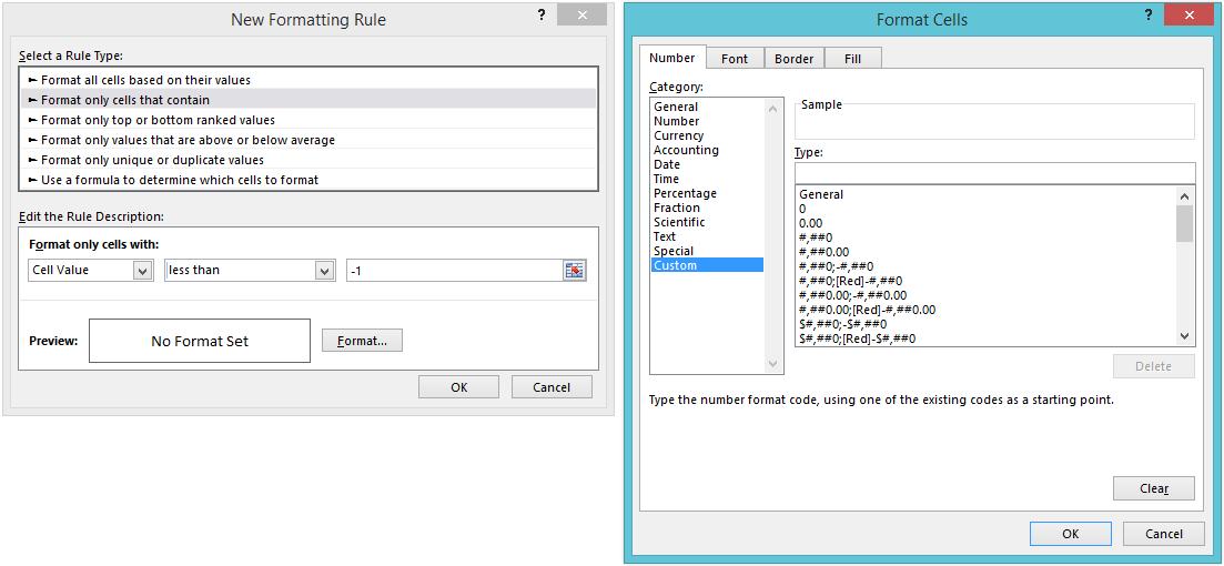
In this above illustration, I have selected conditional formatting to occur if the value in the cell is less than -1.  Pressing the ‘Format…’ button then allows the user to select how the number formatting might appear.

Other conditional number formats may be added to the same cell(s) so that one cell may have values appear as follows:

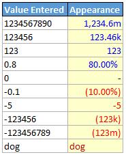
To do this, I would:

• construct the underlying number formatting first.  Personally, I would use custom number formatting so that all positive and negative numbers appeared as percentages, zero as a hyphen (“-“) and text as displayed above;
• next, I would apply conditional formatting number formatting where the cell value is greater than one so that numbers greater than a million could be displayed to the nearest 0.1m, numbers less than a million but greater than or equal to 1,000 could be displayed to the nearest 0.00k and numbers lower than 1,000 (but necessarily greater than one) could be displayed as integers
• finally, I would apply a second set of conditional formatting where the cell value is less than -1 as required.

I do not go through the required syntax here.  My suggested solution can be found in the attached Excel file (below).

Since many, many conditional formats may be applied to one cell in Excel, you can soon apply significantly more than four formats to any cell(s) in Excel.  Brilliant. 

One tip though: always try to add conditional formatting after completing all of the calculations in your model.  This is because conditional formatting sometimes misbehaves when rows or columns are deleted and / or inserted.  Trust me, it’s less work to add it at the end!