Modelling Actual versus Budget

In this article we look at how to structure models effectively and efficiently in order to keep track of actual data versus the original budgeted / forecast information. By Liam Bastick, Director with SumProduct Pty Ltd.

Query

I have to keep track of how actual data compares to the original budget / forecast data and report the variances. Do you have any tips as to how to structure my spreadsheet?

Advice

This is an area where I have seen modellers get into a mess with alarming regularity. However, with a little thought at the outset, the OFFSET function (see also the following link) can prove very useful.

OFFSET Remembered

As a reminder, the syntax for OFFSET is as follows:

The arguments in square brackets (Height and Width) can be omitted from the formula and will be for the entirety of this article.

In its most basic form, OFFSET(Ref,x,y) will select a reference x rows down (-x would be x rows up) and y columns to the right (-y would be y columns to the left) of the reference Ref.

To assist with this topic, please feel free to download the following attached Excel file.

Setting Up the Original Budget / Forecast Data

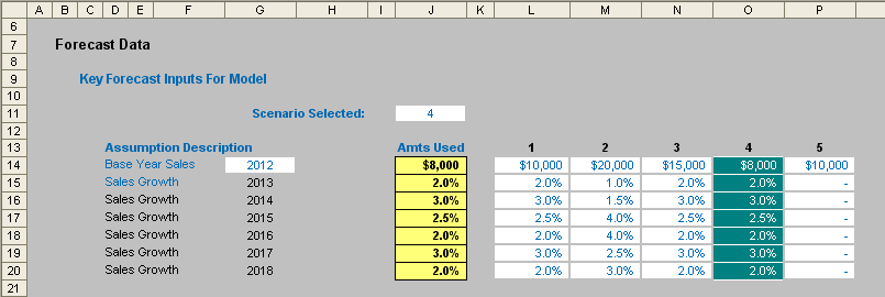
This can simply be typed in, but given the what-if analysis demanded of most finance professionals these days, I would be tempted to set it up in a scenario table, viz.

This method allows for various scenarios to be modelled easily with a different set of input data inserted into each column (from column L onwards in this illustration). A selector (cell J11 in the figure above) is used to select the active scenario, which may be highlighted using conditional formatting (see the following link).

The data used to drive the model is then highlighted in column J (here, emphasised in yellow) using the follow formula for cell J14 for example:

In other words, this formula looks up data x columns to the right of column K, where x is specified as the value input in cell J11 (here, this value is 4 so column O’s data is selected).

Clearly, using a columnar approach here makes it very straightforward to set the various scenarios out. However, most financial models are displayed with dates going from left to right across columns rather than down the page using rows. This requires us to transpose the data, and again we may use OFFSET to ‘flip’ the data:

Here, the period numbers specified in row 31 make it easy for us to transpose the data. For example, the formula in cell L34 would be:

i.e. insert the data x rows down from cell J13 in the first graphic, where x is again specified as the value input in cell J11.

Take care, however, if using an amount followed by growth rates approach for forecast / budget data. The amounts using these examples should be as follows:

The correct formula here is:

for cell L36 (say), i.e. if it is the first period take the amount, otherwise take the amount calculated in the preceding period and multiply it by (1 + growth rate specified in the current period not the next period).

Including Actual Data

When actual data is input into a model, frequently it replaces the original information, and therefore management loses the ability to see how accurate forecasts were originally and how budgeting may be improved.

One way round this would be to simply have “Actuals” as one of the scenarios so that all forecasts are retained. This is often all that is required, and if so, simply do that – Keep It Simple Stupid (KISS).

However, often we may wish to undertake variance analysis by comparing actual data with the original budgeted information. In this case, I would suggest the following approach.

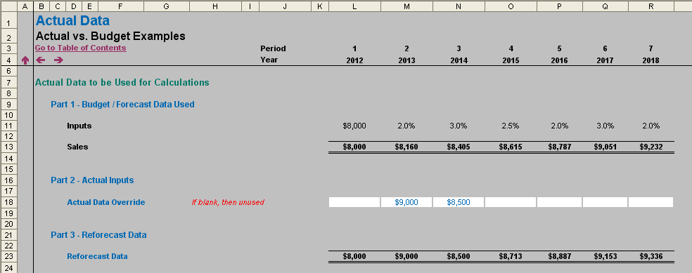
Rows 9 to 13 of this illustration simply reiterate the calculations already detailed above regarding the original forecasting.

Note row 18 however: this is where actual data is added instead. In my example, I simply use hard coded inputs for my data, but it only requires a simple variation to this methodology to revise growth rates, etc.

Using my logic, we simply use actual data where it is available; otherwise we fall back on the original data and calculations. This is achieved by the formula in row 23 in my example, which is (for cell L23):

i.e. if there is data in the corresponding cell in row 18 use it; if not, if it is the first period take the original input value, otherwise simply inflate the prior period amount by (1 + growth rate for that period). It may include a nested IF statement, but it is still a relatively simple and straightforward calculation.

Presentation of the Outputs

Performing the calculations is only half of the battle. Modellers often have difficulty comparing the original outputs with the reforecast counterparts in an effective and efficient manner. If sufficient, the following would be relatively straight forward:

This is very easy to put together, but alas, more often than not, the following presentation is required by senior management instead:

Seem familiar? I have been a model reviewer for many a year and seen this type of output on an extremely regular basis. Many senior management teams like it this way and it is not my role to challenge the status quo – well, at least not on this forum anyway!

The problem with this layout is that it lends itself to promoting poor practice. Modellers tend to a large number of unique formulae across a row, which in turn slows down model construction and increases the potential for mistakes, such as referencing errors.

If you have to use this layout, creating the simple summary elsewhere (maybe on an input page),

inserting two additional lines on the output sheet and using the OFFSET function once more may make your potential troubles a thing of the past, viz.

The interim calculation is straightforward, summarising the original calculations, the revised calculations and the difference (variance) between them.

If you inspect the attached Excel file, you will see that each row of the revised output example contains only one unique formula copied across, making it easy to edit, extend and review. This is achieved by adding two rows:

• Selector (row 7): identifies whether the column should be reporting the budget information, the actual data or the variance. The equation used makes use of the MOD(Number,Divisor) function (see the following article):

• List_Depth is the number of selections (Budget, Act / Ref’cast, Variance) permissible – in this case three. =MOD(L$4,List_Depth) takes the counter and converts each one to 1, 2 and zero (i.e. the remainder upon dividing the counter by three). The remainder of the calculation, +IF(MOD(L$4,List_Depth)=0,List_Depth,0), simply forces a zero to three instead, so that the Selector gives the values 1, 2 and 3 alternately.
• Year No. (row 8): simply notes which year the column is reporting using the formula:

• i.e. the year increases the period after the counter is a multiple of three (in this example). Using List_Depth as a variable means that this idea can be easily extended to summarise other data such as reforecasts, % differences etc. (i.e. have different periodicities).

Therefore, in my example, row 13 requires a very simple formula to generate the required outputs:

BC_Sales_Summary is a range name (see the following article) where BC stands for ‘Base Cell’ and in my example would be cell K28 in the Interim Calculation illustration. The reference would then be offset by Selector number of rows (e.g. if the value of Selector were 3 it would reference the Variance row) and by Year No. number of columns (e.g. if the value of Year No. were 2 it would refer to the 2013 data). For example, cell Q13 equals

which would refer to the 2013 Variance figure $840.

Easy!

This idea can be extended very simply using range names for greater transparency. Please see the attached Excel file for further details.