Dealing with Multiple Criteria

This article deals with a recurrent themem in modelling: summarising data that meets multiple criteria. By Liam Bastick, director with SumProduct Pty Ltd.

Query

I want to summarise the sales made by my business that meet various criteria (e.g. sales for a particular region for a particular product).  SUMIF only works with one criterion.  Due to end user requirements I don’t wish to use PivotTables: is there any way I can obtain the analysis by using a formula?

Advice

This is an example of conditional summing, i.e. where you wish to add numerical values provided they meet certain criteria.  For example, imagine you were reviewing the following data summary:

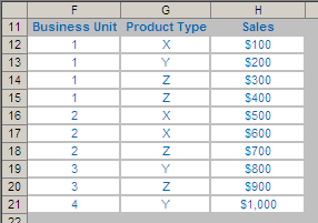
The function SUMIF(range,criterion,sum_range) is ideal for summing data based on one criterion:

• range is the array that you wanted evaluated by the criterion (in this instance, cells F12:F21)
• criterion is the criterion in the form of a number, expression, or text that defines which cell(s) will be added, e.g. “X”, 1, G26 or “<>”&G27 (this last one means ‘not equal to the value in cell G27’)
• sum_range are the actual cells to be added if their corresponding cells in range match the criterion.

So, to find the sales for Business Unit 1 in the above example, we would type =SUMIF(F12:F21,1,H12:H21) (which is $1,000), or to find the total sales of Product X we might type =SUMIF(G12:G21,”X”,H12:H21) (which is $1,200) (note that the text must be in inverted commas).

This month’s problem can be expressed as follows, how would you find the total sales of Product Z in Business Unit 1 using a formula?  That’s two criteria and SUMIF will not work with multiple conditions.  Fortunately, there are several alternatives.  For once, I am going to stick with Excel 2003 and earlier because there is a SUMIFS function in Excel 2007 that resolves our query in seconds:

The issue here is that this function is new to Excel 2007 and is therefore not backwards compatible with earlier versions of Excel.  Hence I will consider other options instead.

Concatenation

It is often possible to cheat with SUMIF by making a ‘mega-criterion’ out of multiple criteria.  This works on joining criteria together usually by using the ampersand (‘&’) operator.

Let’s consider our example, slightly revised, from above.

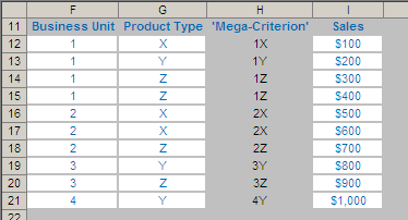
A new column has been inserted (column H), with a formula combining the contents of columns F and G (e.g. the formula in cell H12 is =F12&G12).  Provided that all possible combinations are unique (i.e. no duplicates can be generated), a simple SUMIF can then be applied, e.g.

This is by far and away the simplest solution – if it works.  It can fall down though (in an other example, the concatenation ”111” might refer to Product 1 in Business Unit 11 or Product 11 in Business Unit 1).

Conditional Sum Wizard

This wizard is not part of the default Excel package: it is an ‘add-in’, i.e. a supplemental program that adds custom commands or features to Excel.  Therefore, unless previously included, this add-in needs to be loaded.  ALT+T+I (Tools -> Add-Ins) is the keystroke that works in all versions of Excel.

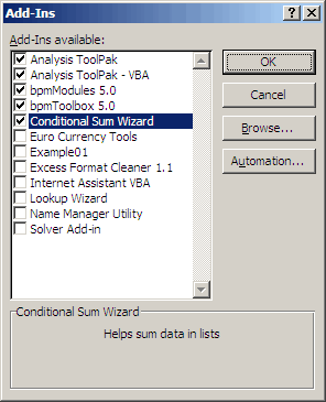
Once loaded, to access it, shortcut keys will not work (ALT+T+C gives rise to a conflict with Tools -> Customize and possibly Tools -> COM Add-Ins).  In Excel 2003 and earlier versions, it can be located on the Tools dropdown menu, whereas in Excel 2007 it is in the final grouping, ‘Solutions’, of the ‘Formulas’ tab.

When activated, the user is prompted by a straightforward multi-step wizard, viz.

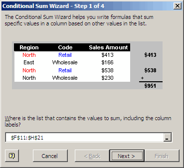
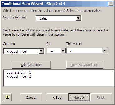
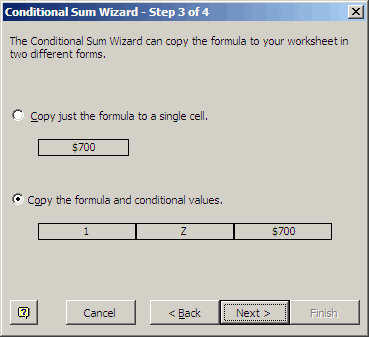
It is recommended that the second option is selected in Step 3, otherwise a formula is constructed containing hard code rather than cell references, giving rise to a ‘static’ rather than ‘dynamic’ formula.  Note that choosing this second option changes the number of steps from four to six.

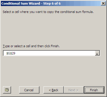
The final three steps simply require where the inputs / outputs should go.

In the example above, you can expect to get a formula similar to the following:

The braces at the beginning and the end of the formula (‘{‘ and ‘}’) cannot be typed in: if the formula had been ‘manually’ generated, you would not press ENTER once the formula is written, but CTRL+SHIFT+ENTER.

This type of formula is known as an array formula.  Array formulae perform multiple calculations on one or more sets of values, and then return either a single result (as in this instance) or multiple results across a range of cells.

Array formulae can be memory intensive and slow down a workbook’s calculation time significantly.  The formulae are not always easy to follow, often exacerbated by the wizard using ‘nested’ functions (i.e. one inside another).  In fact, with a little practice, it is often possible to write simpler, more efficient array formulae without the wizard.

But it’s a great place to start!

DBASE Functions

Perhaps one of the lesser known families of Excel functions is the DBASE family, e.g. DSUM, DMAX, DMIN.  Working similarly to their ‘non-D’ counterparts, these functions interrogate a database in a reasonably transparent way.

The key function for our query is DSUM(range,field,criteria):

• range is the entire array that you wanted evaluated by the criteria (in our example, cells F12:H21, i.e. the whole table where the first row must be the headings / column labels)
• field is the column heading cell reference, the column heading typed in inverted commas, or a number (without the quotation marks) which represents the position of the column within the array (1 for the first column, 2 for the second column, etc.).  In this instance field could be H11, “Sales” or 3
• criteria is the range of cells that contains the conditions to be specified.  This can be highly flexible (the same heading can be used more than once for instance) as long as it includes at least one column label in the top row and at least one cell below each column label in order to specify the condition

From our example above, the following could be a criteria table:

Our formula in this case would be DSUM(F11:H21,3,F26:G27) (=$700).

More than one row can be used.  Criteria put in the same row are ‘AND’ criteria, so in our example above, to be summed, the Business Unit must be 1 AND the Product must be Z.

If more rows were added, each row is read as ‘OR’ criteria.  For example:

Here, all sales are sold which relate to Business Unit 1 OR Product Z (=$2,600).

DBASE calculations are like ‘halfway houses’ between formulae and pivot tables (that do not refresh automatically if data / assumptions are changed).  Once mastered, they are fairly easy to construct and are quite transparent for users and developers alike.  Unlike SUMIF and the Conditional Sum Wizard, OR criteria can easily be selected too.

Their main drawback here is if multiple results are required.  The criteria tables needed may add significantly to the overall file size and confuse users as to which criteria table relates to which formula.

SUMPRODUCT

I must admit this is my favourite function in Excel (hence the company name).  For those who do not know it, SUMPRODUCT(array1*array2*…) appears quite humble upon first glance.  Consider the following sales report:

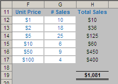
The sales in column H are simply the product of columns F and G, e.g. the formula in cell H12 is simply =F12*G12.  Then, to calculate the entire amount cell H19 sums column H.  This could all be performed much quicker using the following formula:

i.e. SUMPRODUCT does exactly what it says on the tin: it sums the individual products.

How does this help the cause?  It is all to do with the properties of TRUE and FALSE in Excel, namely:

• TRUE*number = number (e.g. TRUE*7 = 7)
• FALSE*number = 0 (e.g. FALSE*7=0).

In our earlier example (repeated below)

we can test columns F and G to check whether they equal our required values.  SUMPRODUCT could be used as follows:

For the purposes of this calculation, (F12:F21=1) replaces the contents of cells F12:F21 with either TRUE or FALSE depending on whether the value contained in each cell equals 1 or not.

Similarly, (G12:G21=”Z”) replaces the contents of cells G12:G21 with either TRUE or FALSE depending on whether the value “Z” is contained in each cell.

Therefore, the only time cells H12:H21 will be summed is when the corresponding cell in the arrays F12:F21 and G12:G21 are both TRUE, then you will get TRUE*TRUE*number, which equals the said number.

Notice that SUMPRODUCT is not an array formula (i.e. you do not use CTRL+SHIFT+ENTER), but it is an array function, so again it can use a lot of memory making the calculation speed of the file slow down.

Used sparingly however, it can be a highly versatile addition to the modeller’s repertoire.  It is a sophisticated function, but once you understand how it works, you can start to use SUMPRODUCT for a whole array of problems (pun intended!).

The following attached Excel file shows examples of all of the above solutions and may help you to choose which solution to use in which scenario.

If you have a query for this section, please feel free to drop Liam a line at liam.bastick@sumproduct.com or visit the website www.sumproduct.com