Multiple Criteria with Errors

This month, in our series of articles providing solutions to common issues encountered by finance professionals, we look at how to deal with errors when using formulae considering multiple criteria.  By Liam Bastick, director (and Excel MVP) with SumProduct Pty Ltd.

Query

How do I deal with errors in data that I am trying to sum up subject to multiple criteria?

Advice

It’s easy to write a formula that will work when everything else is working perfectly.  It’s much more challenging to write a formula that will work when our data doesn’t work the way we want it to.  To start this new year, we’re going to talk about adding up values when we have text and other nasties.

We’ve covered how to do sums with multiple criteria using the SUMPRODUCT function before.  However, this doesn’t work if we have text or errors in our data.  Consider the following example:

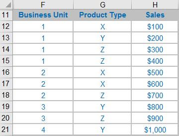
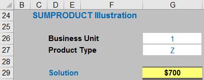
This is reasonably straightforward.  Here, I compare the Business Unit to the input, the Product type to the input, and then multiply the results by the values to get:

If you’re a regular reader of the Spreadsheet Skills section, this will have been easy so far; if not feel free to consult my past article here.  However, not all data behaves nicely:

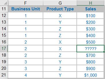
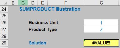
With text in a cell, our function is attempting to multiply “?????” with 1s and 0s, which leaves us with #VALUE!, which is not the desired result.  If only there were a way to ignore text or errors..?

Enter SUMIFS.  SUMIFS has the nifty feature that it will ignore text values in the vector that we are summing, just like the SUM function.  It behaves like SUMIF (see this article for further details) just for multiple criteria rather than a single criterion.  I can replace the SUMPRODUCT function with SUMIFS like so:

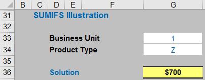
Here, the formula is:

This solution ignores the text whether it forms part of the answer or not.  Since SUMIFS will use the conditions to isolate only matching values that should be summed, it also has the benefit of ignoring items like #N/A in unused data that may cause errors. 

Do note that if the #N/A result occurs in the data, there are other ways to get around this issue.  Did you know that you can incorporate error results into your conditions?  You could try the following for example:

The last argument ensures that the #N/A results will be ignored, regardless of whether they form part of your target data.  You could repeat this with any other error results as well, though this may result in a very long formula if you don’t consider shortcuts!

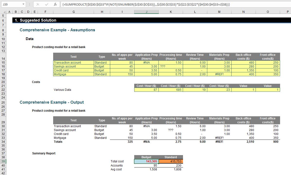
Suggested Solution

This image is a screenshot from the attached Excel file, which contains my suggested solution.  This file has had some issues with data and some of our inputs have become garbled (no change there then).  

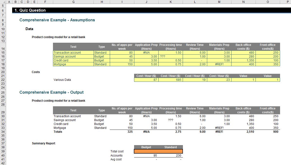
A very “basic” solution would be the following wonder:

Lovely.  It works, but it’s far from pretty.  Sounds like me. 

The N function returns the value of any contents that appear to be numbers and treats text as zeros and errors as errors.  It’s a “brute force and ignorance” approach but it does appear to get the job done.  The problem is, what if (a) I add more rows and / or columns and / or conditions and (b) I don’t have a spare six hours to understand how the formula works?  It’s very simple to miss a cross-multiplication too.

No, I suggest the following – much shorter – solution instead:

It’s a short, “simple” array formula (one that requires entering using CTRL + SHIFT + ENTER, please see this article for more details) – don’t try typing in the brace brackets ({ and }) yourself.

Last time I explained how errors / text could be ignored when data is in a row or a column (“vectors”) using SUMIF or SUMIFS.  However, my question deliberately used multiple rows and columns (an “array” of data) because these useful functions will not work in this instance.

Our old friend SUMPRODUCT comes to the rescue in this instance.  For a refresher on SUMPRODUCT, please see this article.  Essentially, the use of the multiplication delimiter is deliberate (the formula will not work if the delimiters were to become commas instead).  It should be noted that this last formula is essentially

where the number of rows in the Column_Vector must equal the number of rows in the Array, and also the number of columns in the Array must equal the number of columns in the Row_Vector.  The Condition dimensions are slightly more relaxed, but typically are similar to either the Column_Vector or the Row_Vector. 

The key trick concerns Array: I must check if the relevant element of the Array contains a number or not.  To be honest, blank cells, text or errors could all create issues in my cross multiplication, so I really want to identify when the cell value is not a number.  This is what

does.  It returns the value in the cell only if it is a number.  After that, it is simply a case of cross-multiplying and adding the array syntax (this is necessary for Excel to consider errors in an array).  If you require more conditions, rows or columns, simply add them.  Easy!

The solution:

{=SUMPRODUCT($I$30:$I$33*IF(NOT(ISNUMBER($J$30:$O$33)),,$J$30:$O$33)*$J$22:$O$22*($H$30:$H$33=J$38))}

is pretty easy to understand once it has been explained to you. 

Word to the Wise

Some readers may have noted that the expression IF(NOT(ISNUMBER(Array)),,Array) appears a little convoluted and could be readily replaced by IF(ISNUMBER(Array),Array,) – which simply swaps the order of the TRUE and FALSE conditions.  That’s true (pun intended), but NOT(ISNUMBER()) is a powerful combination that comes up time and time again in Excel error testing (e.g. to highlight cells that do not contain numbers using conditional formatting).  Therefore, my use of NOT() to negate TRUE and FALSE was deliberate so that you know how to report by exception.

If you have a query for the Spreadsheet Skills section, please feel free to drop Liam a line at liam.bastick@sumproduct.com or visit the SumProduct website.