Opting for Optimised Economic Life

When modelling for accounting purposes, sometimes you need to verify the life chosen for depreciation purposes (in most jurisdictions, taxation reporting does not have this requirement, so lives for tax purposes may be simply be assumed).  This cannot be just “any” number: it is supposed to reflect the economic life.

The definition of economic life is stated as the timespan over which the annual cost of owning and operating a non-current asset (held for continuing use in the business) is minimised.  The economic life of such an asset can be a function of factors such as physical wear and tear, usage and technological obsolescence.

To establish what constitutes minimum costs, I want to consider not only the costs incurred but the timing of them too – discounted cash flows to the rescue!

The easiest way to explain this is with an illustration.  This example is contained in the attached Excel file.  Assume I have the following forecast cost data:

For this non-current asset, I have three cost categories, forecast for each of the next eight years (you may need to project further in real life).  You should note that the Purchase Price is the cost to buy a new, replacement asset in x years from now – not the purchase price to buy the asset now.  That figure is both sunk and / or decision irrelevant as we are assuming we already possess the asset.

I assume Maintenance Costs will be incurred each year.  To keep the (discounted) cash flow simple, I will assume the costs are incurred at the end of each period too (not an unreasonable assumption to make as businesses will often try to keep their costs to a minimum and tend to delay costs where they can).

Assuming we replace this asset after eight [8] years, a discounted cash flow financial appraisal would look something like this:

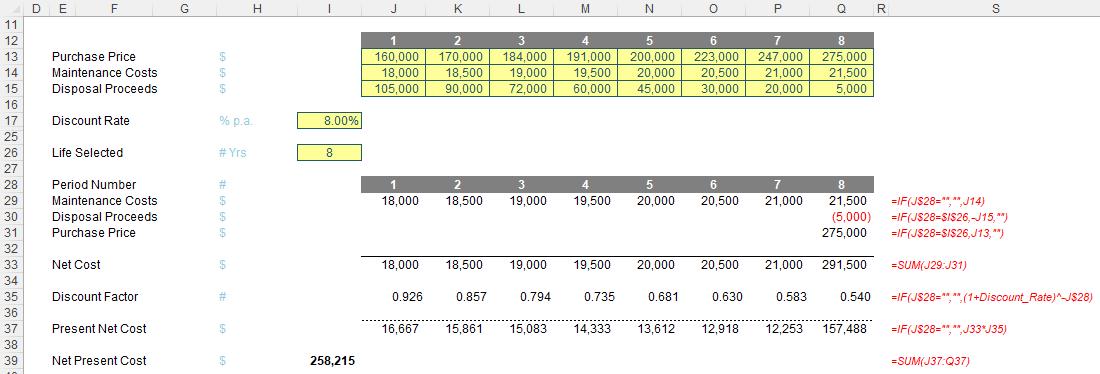
Do note that I ignore tax, as this would be an assumed constant and again, is decision irrelevant.  What you might see in these straightforward calculations is several IF statements that cut off costs after so many periods, or only display them for a particular period.  That is so I may vary the life assessed.  The discount rates are simply taken assuming cashflows occur at the end of each period, e.g. for time n, the discount factor would be

or

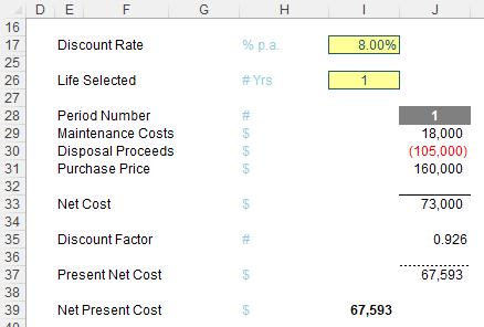
For example, this would be the Net Present Value (NPV) / Net Present Cost (NPC) for one year:

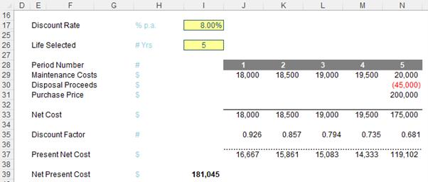
For five years, the calculation would be:

Obviously, the costs appear to increase each year, as there will be additional Maintenance Costs, Disposal Proceeds will reduce and the Purchase Price will increase.  On that basis, we should replace assets once every picosecond, but that’s not exactly viable.  Besides, it would be wrong.

We need to calculate what the average annual cost is.  Simply dividing by the number of periods would be incorrect as we are discounting the cashflows.  We need to take this into account.  Therefore, we weight this average by diving by the sum of the discount factors instead (known as the cumulative discount factor):

Our initial eight-year appraisal would then become:

whereas the one-year assessment would be:

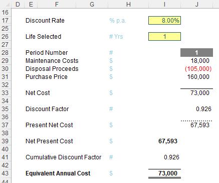
Clearly, eight years would be a better bet than one year, on this basis.

Rather than estimate the economic life by performing a “manual goal seek”, I can derive the optimum figure using Data Tables.  But first, let me provide a reminder.

Data Tables Recap

I have discussed Data Tables previously, so I will focus on the salient points required.  This is best illustrated using an example similar to the one I am constructing here:

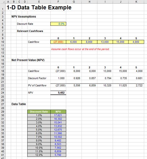
It’s not vital you understand what this spreadsheet is doing.  It is using inputs in cells F5 and F10:K10 to generate an output in cell K24, as it calculates what cash received in row 10 would be worth now if interest were 8.0% per period.  But what if I wanted to know how the output (NPV) would change if I varied the input discount rate?

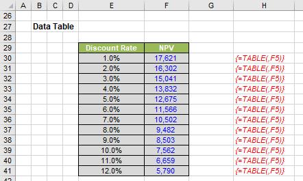
It is quite easy to construct a table (a Data Table) similar to the one displayed in cells E29:F41above.  The required discount rates are simply typed into cells E30:E41, but the heading in cell F29 is not what it seems.

For a 1-D Data Table to work using a columnar table similar to the one illustrated, the top row of the second and any subsequent columns has to contain the reference to the output cell(s).  Many modellers will do this, putting the headings in the row above instead and then they may or may not hide this row in order to compensate.

There is a crafty alternative (employed above). Using CTRL + 1, ALT + H + O + E or select ‘Format Cells…’ from the ‘Format’ drop-down in the ‘Cells’ grouping of the ‘Home’ tab of the Ribbon to ‘Format Cells’.  Then, if we go to the ‘Number’ tab we can still type the formula(s) in but change the outward appearance of the cell.  It is with this borne in mind that cell F29 is formatted as follows:

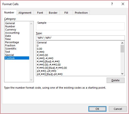
Here, I have typed in “NPV”;“NPV”.  Essentially, what I have done here is replaced all non-negative numbers with the text “NPV” and negative numbers with the text “NPV”.  You might wonder why I have I typed this in twice?  If the number is negative and the second “NPV” has not been defined the negative number would be replaced by “-NPV” instead – which is not what we want.

Once this formatting has been done and the formula

has been typed into the header in cell F29 (giving it the appearance “NPV”, then select cells E29:F41 and go to ‘Data Table…’ in the What-If Analysis drop-down list in the ‘Forecast’ grouping of the ‘Data’ tab on the Ribbon (Alt + A + W + T):

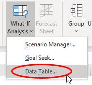
This calls the ‘Data Table’ dialog box:

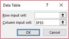
At this point, confusion often sets in as users are often unsure whether they should be entering details in the ‘Row input cell:’ and / or ‘Column input cell:’ input boxes.  The rules are quite simple:

• referenced directly, the inputs and outputs must be on the same sheet as the Data Table (although there are ways and means around this)
• use only one input box if you want to flex one input; use both if you wish to flex two
• if inputs are in a column in the Data Table, use the ‘Column input cell:’ input box
• if inputs are in a row in the Data Table, use the ‘Row input cell:’ input box.

Here, my inputs are in a column and I want to use them to substitute for the value in cell F5, so I select cell F5 for the ‘Column input cell:’ input box.  Clicking ‘OK’ results in the following summary:

Returning to the Economic Life Calculation

Now we have an appreciation of Data Tables, I may construct a simple summary as follows:

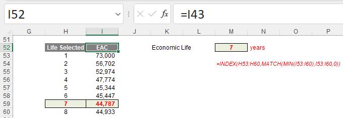
Note that I have put the formula =I43 in the header cell I52, then highlighted the range H52:I60 before creating the Data Table.  This shows that for the costs forecast, the economic life for this asset should be seven (7) years, viz.

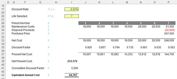
With the correct set-up, this economic life verification becomes trivial and should therefore be performed at least once a year, in order to confirm the appropriate accounting policies, etc.

Word to the Wise

Sometimes, you may find all of the numbers in your Data Table are identical.  If this happens, you need to check your calculation settings.  To do this, go to Excel Options (File -> Options or ALT + F + T) and then select ‘Formulas’.  In the ‘Calculation options’ section, please ensure the ‘Workbook Calculation’ is set to ‘Automatic’:

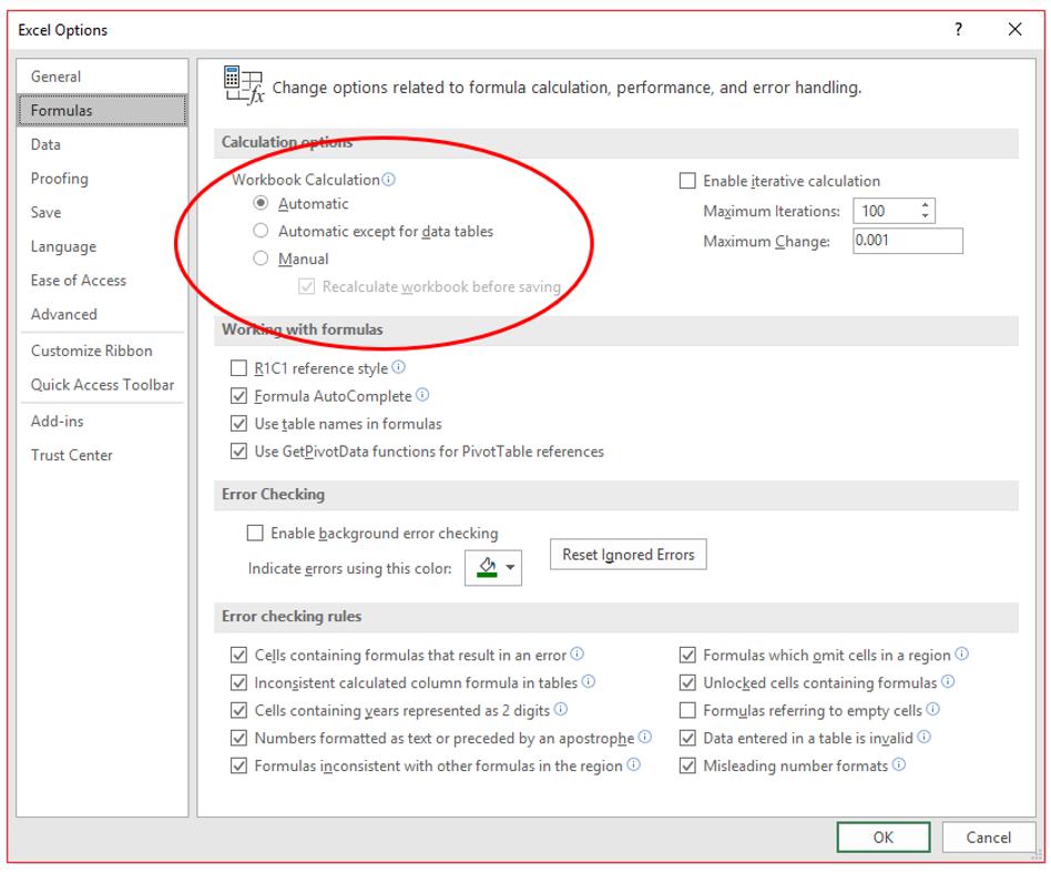
Any other setting will not calculate Data Tables correctly.  The reason for this is Data Tables can consume a significant amount of memory and slow down workbook calculations – hence the options to disable them.