Pivotal Pivot Tables

This article looks at how to turn data in Excel into information using PivotTables. By Liam Bastick, director with SumProduct Pty Ltd.

Query

I work with large tables of data which I need to interrogate on a regular basis. A work colleague suggested I set up a PivotTable. However, I’m an Excel novice and unsure how they work. Could you give me some guidance please?

Advice

A PivotTable is a semi-dynamic, tabular summary of data. It is one of Excel’s most flexible tools and can provide results that would take some time to reconstruct with sophisticated uses of functions such as SUMIF, SUMPRODUCT, etc.

Excel 2007 has increased PivotTable flexibility significantly from earlier incarnations. However, as with many pre-Excel 2007 features, the location of various tools and options needs to be re-learned. This article provides a basic overview for both Excel 2003 (and earlier) users as well as Excel 2007 users.

In order to get to grips with the basics of a PivotTable, I am going to use the attached Excel file example.

In this illustration, imagine we are a Head Office Analyst reviewing the electrical sales of four stores: imaginatively called North, South, East and West.

Creating a PivotTable on the same worksheet is fairly straightforward, albeit a little different between the Excel versions. If the database is in one block (a ‘contiguous’ range), simply select any cell within the database and then:

Excel 2003 and earlier	Excel 2007
Load up the Pivot Table Wizard, Data -> PivotTable and PivotChart Report… (ALT + D + P) In Step 1 of 3 of the Wizard, choose ‘Microsoft Office Excel list or database’ as the data that you want to analyse and also select PivotTable as the report you want to create In Step 2, confirm that the entire selection of data has been identified In Step 3, put the report in the ‘Existing Worksheet’ and, say, choose cell L9 The layout can be detailed by selecting the ‘Layout’ button in the Wizard, but for this example we will click on ‘Finish’ instead	The Pivot Table Wizard does not appear to exist in Excel 2007, but if you select the keystrokes (ALT + D + P), the dialog box will indeed pop up albeit with restricted functionality Consequently, it is probably easier to insert a Pivot Table from the Insert tab of the Ribbon, then click on the PivotTable icon, and then select PivotTable The Create PivotTable dialog box appears. Choose ‘Select a table or range’ and confirm the entire selection of data has been identified For placement, select ‘Existing Worksheet ‘and choose, say, cell L9 Click ‘OK’ (layout cannot be constructed in a dialog box)

Excel 2003 and earlier

Excel 2007

Load up the Pivot Table Wizard, Data -> PivotTable and PivotChart Report… (ALT + D + P)
In Step 1 of 3 of the Wizard, choose ‘Microsoft Office Excel list or database’ as the data that you want to analyse and also select PivotTable as the report you want to create
In Step 2, confirm that the entire selection of data has been identified
In Step 3, put the report in the ‘Existing Worksheet’ and, say, choose cell L9
The layout can be detailed by selecting the ‘Layout’ button in the Wizard, but for this example we will click on ‘Finish’ instead

The Pivot Table Wizard does not appear to exist in Excel 2007, but if you select the keystrokes (ALT + D + P), the dialog box will indeed pop up albeit with restricted functionality
Consequently, it is probably easier to insert a Pivot Table from the Insert tab of the Ribbon, then click on the PivotTable icon, and then select PivotTable
The Create PivotTable dialog box appears. Choose ‘Select a table or range’ and confirm the entire selection of data has been identified
For placement, select ‘Existing Worksheet ‘and choose, say, cell L9
Click ‘OK’ (layout cannot be constructed in a dialog box)

Notice that cell L9 is not the top left of the PivotTable, as you would expect. In fact, L7 (same column, two rows higher) is the first cell for the Page Field insertion (see figure below). When selecting where to place a PivotTable, always remember to select a cell two rows further down than you might otherwise think.

PivotTable Construct

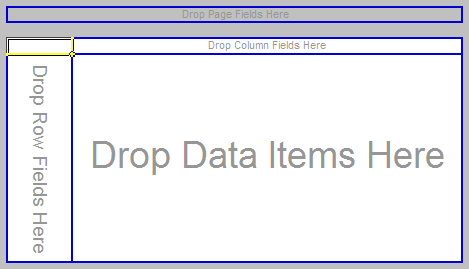
The PivotTable has four areas where data fields may be placed (a data field is simply any one of the columns of the database, e.g. Date, Store, Item in this example):

Page: Values in this field appear as page items in the PivotTable;
Row: Values in this field appear as row items in the PivotTable;
Column: Values in this field appear as column items in the PivotTable; and
Data: The field to be summarised – if this data is numerical in nature, SUM (how much) will be the default operation, otherwise COUNT (how many) is used. They are easily changed, by double clicking on the dragged field and changing SUM to AVERAGE or COUNT, etc.

PivotTable Construct

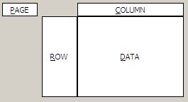
More than one field can be placed in any of these locations – the effect is a hierarchical grouping depending upon the order of placement.

In essence, a PivotTable is a three-dimensional summary of a database. Consider it as a book: each page has a summary table of a selection of the data (for instance, in our example, each page could show the sales of each electrical item for each store on a particular date, so Page 1 is 1 April, Page 2 is 2 April, etc.).

To populate the layout, it is simply a case of dragging and dropping. How this is done exactly depends on which version of Excel you have:

Excel 2003 and earlier	Excel 2007
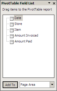
Once the PivotTable has been inserted, the PivotTable toolbar should appear (if not, from the dropdown menu, select View -> Toolbars -> PivotTable) The PivotTable Field List dialog box should also appear (if not, right click on the layout and select ‘Show Field List’ from the shortcut menu The fields can be dragged on to the layout using the mouse, or simply select a field in the dialog box window and then make a choice from the drop down box and click ‘Add To’ In this example, Date is to be placed in the Page Area	Instead of a toolbar, two additional tabs are added to the end of the Ribbon – when the PivotTable is selected – Options and Design The PivotTable Field List window pane should also appear (if not, click on the Field List icon in the Show / Hide section of the PivotTable Tools Options tab) The fields can be dragged on to the layout using the mouse, or simply select a field in the top dialog box window and drag it into one of the four windows below (‘Report Filter’ is the ‘Page Area’ equivalent) In this example, Date is again to be placed in the ‘Page Area’

Excel 2003 and earlier

Excel 2007

Once the PivotTable has been inserted, the PivotTable toolbar should appear (if not, from the dropdown menu, select View -> Toolbars -> PivotTable)
The PivotTable Field List dialog box should also appear (if not, right click on the layout and select ‘Show Field List’ from the shortcut menu

The fields can be dragged on to the layout using the mouse, or simply select a field in the dialog box window and then make a choice from the drop down box and click ‘Add To’
In this example, Date is to be placed in the Page Area

Instead of a toolbar, two additional tabs are added to the end of the Ribbon – when the PivotTable is selected – Options and Design
The PivotTable Field List window pane should also appear (if not, click on the Field List icon in the Show / Hide section of the PivotTable Tools Options tab)

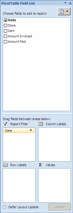
The fields can be dragged on to the layout using the mouse, or simply select a field in the top dialog box window and drag it into one of the four windows below (‘Report Filter’ is the ‘Page Area’ equivalent)
In this example, Date is again to be placed in the ‘Page Area’

Using the Field List, drag the Date field into the Page Area, the Store field into the Row Area, the Item field into the Column Area and the Amount Invoiced field into the Data Area (Values in Excel 2007), viz.

Example PivotTable 1

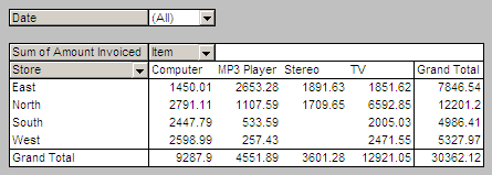
The power of the PivotTable should already be apparent. From the humble origins of a list of data, we can now see which store is leading in sales, enquire why there are no stereo sales in the South West and so on. Using the drop down arrows in the table (you may need to make them visible in Excel 2007, PivotTable Tools -> Options -> Field Headers icon) or in the Field List pane in Excel 2007, we can filter for certain selections, e.g. North’s sales on 2 April:

Example PivotTable 2

But let’s not stop there.

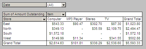
Resetting the PivotTable, one key report would be to determine the amounts outstanding. To do this, we need to construct a calculated field:

Excel 2003 and earlier	Excel 2007
In the PivotTable toolbar, select PivotTable -> Formulas -> Calculated Field… (ALT + P + M + F)	In the Ribbon, select PivotTable Tools, Options tab, then click on the Formulas icon in the Tools section and click on Calculated Field

Type ‘Amount Outstanding’ in the Name Field (note it can be modified later)
Clear the Formula box and type ‘=’ then select ‘Amount Invoiced’ from the Fields window and then click ‘Insert Field’
Type ‘-’ then select ‘Amount Paid’ from the Fields window and then click ‘Insert Field’

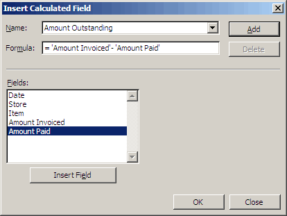
Insert Calculated Field Dialog Box

Click the ‘Add’ button and then ‘OK’.

As a consequence of doing this, Excel may ask whether you want the destination cells to be replaced (the software thinks you want to replace or add to the Data Field). Rather than worry about choosing ‘Yes’ or ‘No’ (obviously, choose one!), simply go to the Field List and de-select the Amount Invoiced field (or drag it off the layout from the top left hand corner) and choose the ‘Amount Outstanding’ calculated field instead:

Example PivotTable 3

One more thing we’ll do while we’re here: the business has a North West division and a South East division. To see how these divisions have performed, we need to group the stores:

Highlight the North and West rows of the table (hold the CTRL key down to select non-contiguous ranges)
Right click and select ‘Group…’ in Excel 2007 or ‘Group and Show Detail’ -> ‘Group’ in earlier versions
The items have been grouped and we have a new, second data field in the Row Area, ‘Store2’ and a ‘Group 1’ grouping:

Example PivotTable 4

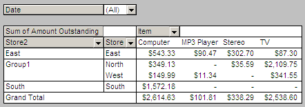
Right clicking on ‘Store2’, we can click on ‘Field Settings…’ and change the name in the dialog box to ‘Division’ and click ‘OK’
Left click on the cell containing ‘Group1’
Go to the Formula bar and change the label to ‘North West Division’
Repeat the process for the South East Division

Example PivotTable 5

This can be collapsed by double clicking on the cell containing the grouping description in all versions or selecting the ‘+’ or ‘-’ symbol in Excel 2007:

Example PivotTable 6

Just an Introduction…

This article was intended only as an introduction to PivotTables – there is plenty more you can do with them. For example:

The PivotTable Options are well worth playing with (Excel 2007, on the Ribbon; earlier versions: from the PivotTable toolbar, choose PivotTable -> Table Options…). It doesn’t take long to spot:
- How to give the pivot table a name
- Adding / removing totals
- Preserving formatting
- Merge labels
Data can be brought in from more than one source
The idea can be extended to pivot charts
Excel 2007 allows even greater functionality, such as 64 levels of sorting rather than 3, more rows and columns and colouring the pivot table more ‘prettily’.

Handle With Care

I mentioned pivot tables were ‘semi-dynamic’ earlier. Pivot tables do not automatically update, i.e. if you change the source data, the data in the pivot table does not automatically recalculate (F9 doesn’t work here). In earlier versions of Excel, if you have more than one pivot table, each pivot table has to be selected and then the refresh icon clicked on the PivotTable toolbar, or PivotTable -> Refresh Data. This is quite cumbersome. However, in Excel 2007, you can refresh them all (in the Ribbon, on the PivotTable Tools Options tab, select the Refresh icon in the ‘Data’ section and choose ‘Refresh All”).
PivotTables can play havoc with underlying worksheet formats (see this example, I have deliberately set it up so that the underlying grey background keeps disappearing)
The Calculated Fields calculations do not always work as intended, especially with ‘*’ and ‘/’: it is a case of “suck it and see”
Get it right though and a pivot table can provide useful analyses that would take half a day to write as a formula (and about the same time for Excel to calculate…).

If you have a query for this section, please feel free to drop Liam a line at liam.bastick@sumproduct.com or visit the website www.sumproduct.com