One, Two, Skip a Few…
Sometimes, modellers find they have to refer to every Nth row – here, we present a simple, error-free way to do this. By Liam Bastick, director with SumProduct Pty Ltd.
Query
I am creating a summary worksheet where I need to produce a block of outputs where each row refers to line items N rows apart. Is there a simple way to do this quickly?
Advice
We seem to have a fixation on Nth items at the moment, but this is a common question. For example, imagine you had sample business data like the following (taken from the attached Excel file):
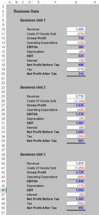
You might wish to create an output which summarises the revenue by business unit. You will need to construct formulae such as =’Business Data’!G10, =’Business Data’!G25, =’Business Data’!G40, … etc.
If you had, say, 500 of these business units you would have a busy but boring morning ahead of you. Surely there is a simpler way that does not require the implementation of macros?
Actually, I can think of two ways of dealing with this common query and I present both solutions below.
Method 1: Text Little Time
This approach requires the first two formulae to be entered into the output sheet as usual, viz.
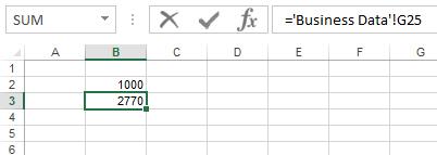
In our example, cell B2 contains the formula =’Business Data’!G10 and cell B3 contains the formula =’Business Data’!G25 (displayed).
Next, edit both formula by typing an apostrophe (‘) before the equals sign in each formula:

Now, these formulae are treated as text and are displayed in the two cells. If you then highlight cells B2:B3 together and copy the formulae down, Excel’s Auto Fill (see Auto Fill Becoming a Drag? for further information) feature will copy the cells similar to below:
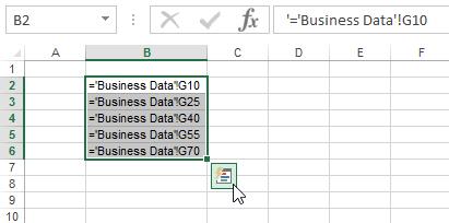
Now, all we need to do is remove the apostrophes. The first idea that comes to mind is to use ‘Replace…’ (CTRL + H) and replace ‘= with =. Unfortunately, this does not work in all versions of Excel as ‘Replace…’ does not seem to recognise apostrophes in certain instances.
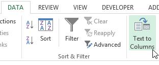
There is a very simple trick to circumvent this problem. With this data still selected, click on the ‘Text to Columns’ button in the ‘Data Tools’ group of the ‘Data’ tab on the Ribbon (ALT + D + E for all versions of Excel or ALT + A + E in Excel 2007 onwards):
This launches the ‘Text to Columns Wizard’ dialog box. In the first step, ensure that the ‘…file type that best describes your data…’ is set to ‘Delimited’:
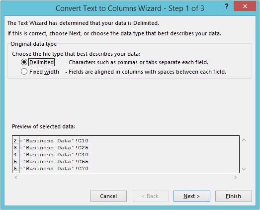
Then, simply depress the ‘Finish’ button. The spreadsheet will then reinstate the formulae, viz.
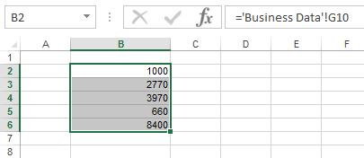
Simple!
Method 2: OFFSET of the Outset
The above approach is fairly simple, but has two major drawbacks:
- This method only works with rows. Using R1C1 formula notation it is possible to create a similar approach for columns, but this technique can be confusing.
- Once the formulae have been reinstated it is not simple to extend the formulae if necessary. This can be cumbersome where the output summaries may differ period to period for example. The OFFSET approach counters these issues. I have discussed OFFSET before (please see Onset of OFFSET for further details).
The syntax for OFFSET is as follows:
OFFSET(Reference,Rows,Columns,[Height],[Width]).
The arguments in square brackets (Height and Width) can be omitted from the formula. In its most basic form, OFFSET(Reference,x,y) will select a reference x rows down (-x would be x rows up) and y columns to the right (-y would be y columns to the left) of the Reference. For example, consider the following grid:

OFFSET(A1,2,3) would take us two rows down and three columns across to cell D3. Therefore, OFFSET(A1,2,3) = 16, viz.

OFFSET(D4,-1,-2) would take us one row up and two columns to the left to cell B3. Therefore, OFFSET(D4,-1,-2) = 14, viz.

Let’s go back to our example:

Note that the Business Unit data is 15 rows apart (e.g. the first block begins in row 8 and ends in row 22, taking the blank rows into account). We can therefore create one formula we can copy down:

In this example, we have started the formula in cell B2 and copied it down to cell B6. The formula in cell B2 is:
=OFFSET(‘Business Data’!$G$10,ROWS(‘Business Data’!$C$8:$C$22)*(ROWS($A$2:$A2)-1),).
The first reference is the Revenue for Business Unit 1. The Rows reference takes the depth of each block (defined here by ROWS(‘Business Data’!$C$8:$C$22)) multiplied by ROWS($A$2:$A2)-1, e.g. in row 2 this factor will be zero, in row 3 it will be 1, in row 4 it will be 2, etc. This ensures that the next Revenue item is referred to in the next row down.
This may seem complex to begin with, but with practice this idea can be adapted for columns to be skipped as well and to allow for other line items (e.g. Gross Profit, Tax) to be selected instead.
Word to the Wise
The attached Excel file demonstrates how data validation (please see >Data Validation for further information) may be used to produce more sophisticated summary reports using just one unique formula:
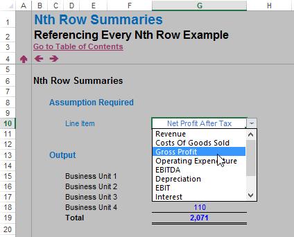
Feel free to download and have a play.
If you have a query for this section, please feel free to drop Liam a line at liam.bastick@sumproduct.com or visit the website www.sumproduct.com

