Simple Pro-Rating Over Time
Some time ago, I wrote about a problem of pro-rating amounts over time, as costs (or revenues for that matter) and reporting dates seldom coincide. In hindsight, I may have over-complicated the fundamental problem by introducing full-time versus part-time and inflationary factors.
I write, “…I may have…” because whilst the article addressed common salary cost issues, it obfuscated a more common problem of just getting pro-rating right. Recently, I have been reviewing various third party financial models where simple errors have been made, and it’s prompted me to address the situation here today.
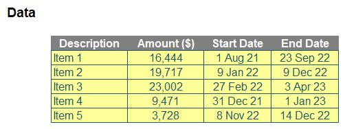
Consider the following simple dataset:

My plan is to allocate these amounts on a daily basis, displayed monthly, for the calendar year 2022. This is really quite simple, but it’s amazing how many times errors are made by the inexperienced.
One of the most common mistakes is actually calculating the number of days in the duration wrong. All too often, modellers will calculate this as
End Date – Start Date
but this is wrong – plain and simple – since this deducts the first day of the duration from the computation. For example, a cost that is incurred on 17 August 2022 would have a start and end date of said date. Therefore, according to the above formula, the duration would be zero [0] days. We must add one [1] to the subtraction:
End Date – Start Date + 1
That’s better. It might be a good idea to add a dates check at this point too:

With the table positioned as in the graphic (above), the error check formula in cell J18 is given by
=IF(OR(I18-H18<0,COUNT(H18:I18)=1),1,)
This checks for two things:
1. The End Date occurs before the Start Date (I18-H18<0)
2. If entered, both dates have been included (COUNT(H18:I18)=1).
This ensures the integrity of the dates data entry.
Now I am in position to calculate the pro-rated amounts on a daily basis, summarised monthly, across the calendar year 2022:

This is one formula copied down and across the entire block. For example, the formula in cell M18 is given by
=IF($I18-$H18>=0,MAX(MIN(M$7,$I18)-MAX(M$6,$H18)+1,0)*$G18/($I18-$H18+1),)
The formula may look a little involved, but it is not that sophisticated:
- MIN(M$7,$I18) calculates the earlier of the final day (M$7) in the period and the End Date ($I18), with anchoring included to ensure the formula may be copied down and across correctly
- Similarly, MAX(M$6,$H18) calculates the later of the first day (M$6) in the period and the Start Date ($H18)
- Therefore, MIN(M$7,$I18)-MAX(M$6,$H18)+1 calculates the number of relevant days in the period. The adjustment of adding one [1] is to ensure the later of the first day in the period and the Start Date is included, as explained earlier
- Calculating the maximum of this and zero, MAX(MIN(M$7,$I18)-MAX(M$6,$H18)+1,0), is computed just to ensure the End Date is later than or equal to the Start Date
- Multiplying by the scalar $G18/($I18-$H18+1) pro-rates the amount ($G18) by the number of days in the period overall ($I18-$H18+1)
- Finally, this is all wrapped in an IF statement, where the formula checks that the End Date is greater than or equal to the Start Date ($I18-$H18>=0), else zero [0] is returned.
That is all that is required, but I add a row total and a final check for completeness, viz.

The row total in column L simply sums the 12 months’ values. However, the ‘Amt Check’ (amount check) in cell K18 (say) requires perhaps some explanation:
=IF(J18<>0,,(ROUND($L18-($G18*(MIN(MAX($7:$7),$I18)-MAX(MIN($6:$6),$H18)+1)/
($I18-$H18+1)),Rounding_Accuracy)<>0)*1)
MAX($7:$7) and MIN($6:$6) calculate the end date and the first date of the calendar year (i.e. 31 December 2022 and 1 January 2022) respectively. Therefore,
MIN(MAX($7:$7),$I18)-MAX(MIN($6:$6),$H18)+1
calculates the total number of days the amounts should be allocated to the year 2022, using similar logic to that detailed earlier. Since $I18-$H18+1 computes the total number of days the amount should be spread across in total, the quotient
MIN(MAX($7:$7),$I18)-MAX(MIN($6:$6),$H18)+1)/($I18-$H18+1)
works out the proportion attributable to 2022 (which will be a value between 0% and 100%). Thus, the multiplication
$G18*MIN(MAX($7:$7),$I18)-MAX(MIN($6:$6),$H18)+1)/($I18-$H18+1)
is the total amount attributable to 2022, and
$L18-($G18*MIN(MAX($7:$7),$I18)-MAX(MIN($6:$6),$H18)+1)/($I18-$H18+1))
represents the difference between the row total ($L18) and this amount calculated. Since Excel may generate rounding errors due to the fact its computations are rounded to so many significant figures,
(ROUND($L18-($G18*(MIN(MAX($7:$7),$I18)-MAX(MIN($6:$6),$H18)+1)/
($I18-$H18+1)),Rounding_Accuracy)<>0)*1
the ROUND function is employed to check that these two values are equal to a given number of decimal places (denoted by the constant Rounding_Accuracy, which is set at five [5] in the attached Excel file).
This formula only makes sense if the dates have been entered correctly, hence the final IF condition that the other check in cell J18 must not have been triggered:
=IF(J18<>0,,(ROUND($L18-($G18*(MIN(MAX($7:$7),$I18)-MAX(MIN($6:$6),$H18)+1)/
($I18-$H18+1)),Rounding_Accuracy)<>0)*1)
Next month, we will be looking at the philosophy of relativistic quantum mechanics and its impact upon Non-Euclidean n-dimensional modular contingencies. (Don’t wait up for that one – Ed.)

