SUBTOTAL – Function and Functionality

Here, we look at a useful but seldom used function / functionality: SUBTOTAL. By Liam Bastick, Director with SumProduct Pty Ltd.

Query

Any tips for including sub-totals in my financial data?

Advice

Data can be sub-totalled in Excel using Excel’s SUBTOTAL() function or the Subtotal functionality. It is important to distinguish between the two features and I will begin with discussing the function.

SUBTOTAL Function

On the face of it, SUBTOTAL seems like many other Excel functions:

The Function_Number is an integer between 1 and 11 inclusive or 101 and 111 inclusive as follows:

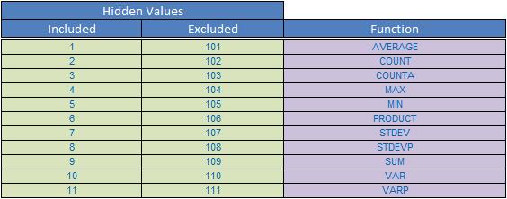
For the Function_Number constants from 1 to 11, the SUBTOTAL function includes the values of rows hidden by the ‘Hide Rows’ command under the ‘Hide & Unhide’ sub-menu of the ‘Format’ command in the ‘Cells’ group on the ‘Home’ tab. These constants should be used when you want to subtotal hidden and unhidden (visible) numbers in a list. For the Function_Number constants from 101 to 111, the SUBTOTAL function ignores values of rows hidden by the ‘Hide Rows’ command. These constants should be used when you want to subtotal the visible numbers in a list only.

If there are other subtotals within Ref1, Ref2,… (or nested subtotals), these nested subtotals are ignored. This is an important feature as it allows you to consider complete ranges without any risk of double-counting.

Please see the attached Excel file for a comprehensive example:

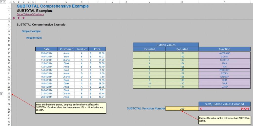
It is a useful function and once you understand how it works with hidden rows and filtering, it can prove to be quite flexible. However, its full power and versatility is not truly realised until you start using the Subtotal functionality…

Subtotal Functionality

To illustrate the power of the Subtotal functionality, I am going to use an example from the attached Excel file, viz.

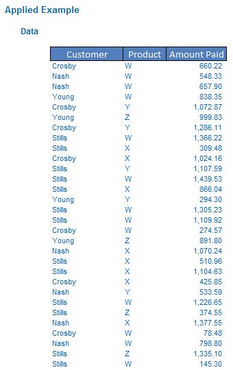
Imagine you have data of sales for four customers and four products over a period of time, which you wish to summarise. Highlighting the table (including the row containing the headers), the data can be sorted using Excel’s built-in Sort functionality (go to the ‘Data’ tab of the Ribbon and then in the ‘Sort & Filter’ section, click on ‘Sort’):

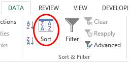
Alternatively, ALT + D + S works for all versions of Excel, too.

This activates the Sort dialog box:

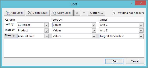
Ensure that the ‘My data has headers’ checkbox has been ticked and then sort as required using the ‘Add Level’ and ‘Delete Level’ buttons as necessary. When finished, click on the ‘OK’ button. The data will have then been sorted:

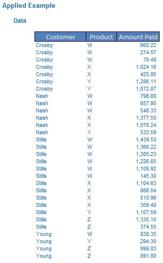
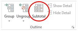
Now the data is in a suitable format for subtotalling. Again, once the data (including the headers) has been highlighted, click on ‘Subtotal’ (located on the ‘Data’ tab of the Ribbon in the ‘Outline’ section):

Alternatively, ALT + D + B works for all versions of Excel, too.

This activates the Sort dialog box:

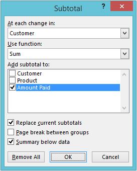
The dialog box is fairly self-explanatory. The SUBTOTAL functions can be used as if you had chosen a Function_Number between 1 and 11. In seconds, you have turned data into information:

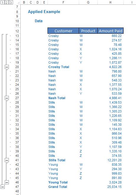
Notice anything? Excel has put grouping in (see Avoiding a Group Protection Racket) automatically.

Please see the attached Excel file for both the Before and After illustrations.

Very useful!

Word to the Wise

If you incorporate filtering in your list / database, the SUBTOTAL function ignores any rows that are not included in the result of a filter, no matter which Function_Number value you use.

It should be noted that the SUBTOTAL function is designed for columns of data / vertical ranges. It is not designed for rows of data / horizontal ranges. For example, when you subtotal a horizontal range using a Function_Number of 101 or greater, such as =SUBTOTAL(109,A1:A10), hiding a column does not affect the subtotal. However, hiding a row in a subtotal of a vertical range will affect the subtotal.

SUBTOTAL is designed only to work on vector references (i.e. where Ref1, Ref2,… are ranges containing wither just one row or just one column). If arrays (ranges of cells containing at least two rows and two columns), SUBTOTAL returns the #VALUE! error value.