Being Dynamic with Variable Hyperlinks
Is it possible to create a hyperlink that can link to different cells? If the answer is no this is going to be a very short article. By Liam Bastick, director with SumProduct Pty Ltd.
Query
I want to create a hyperlink within my workbook that will link to different cells depending upon certain conditions. Is this possible?
Advice
Regular readers of these articles will have noted that I commonly use hyperlinks in my Excel files as they are a great way to move around a file. Once you know how to construct them, they take seconds to insert.
I have talked about hyperlinks before (please see Hyperlinking Chart Sheets for further details). Essentially, the ‘Insert Hyperlink’ dialog box is fairly straightforward to use and readily accessed via one of two keyboard shortcuts, either ALT + I + I or CTRL + K. Alternatively:
Excel 2003 and earlier
- From Insert drop down menu, select Hyperlink
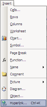
Excel 2007
- From the Ribbon, select the Insert tab and click on the Links group

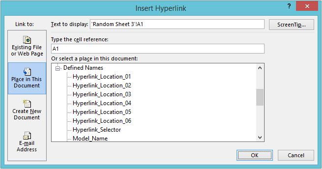
To create a hyperlink, first select the cell or range of cells that you wish to act as the hyperlink (i.e. clicking on any of these cells will activate the hyperlink). Then, open the Insert Hyperlink dialog box (above) and select ‘Place in This Document’ as the ‘Link to:’, which will change the appearance of the rest of the dialog box.
Insert the text for the hyperlink in the ‘Text to display:’ input box (clicking on the ‘ScreenTip…’ macro button will allow you to create an informative message in a message box when you hover over the hyperlink).
The next two input boxes, ‘Type the cell reference:’ and ‘Or select a place in this document:’, work in tandem – sort of:
- If you type a cell reference in the first input box without making a selection in the second input box, the hyperlink will link to the cell reference on the current (active) worksheet;
- If you type a cell reference in the first input box and select a worksheet reference in the second box, the hyperlink will link to the specified cell in the given worksheet. In my example above, this hyperlink will jump to Sheet1 cell A1; or
- If you select a ‘Defined Name’ (i.e. a pre-defined range name) in the second input box, this will link to the cell(s) specified. This is the recommended option, where available, if you wish to link to cell(s) on another worksheet within the same workbook. This is because if the destination worksheet’s sheet name were to be changed, the link would still work.
It is recommended that range names are used for the destination so that the hyperlink will work if the worksheet name to which the link points is changed.
This methodology is fine, but what happens if you want the hyperlink to point to different places depending upon certain conditions? It is actually quite simple, but requires the modeller to use the HYPERLINK function rather than the Insert Hyperlink methodology described above. Let me illustrate with a simple example.
Example
Here, the intention is to create a variable hyperlink, often referred to as a dynamic hyperlink. For the purposes of this illustration, please refer to the attached Excel file example. In this instance, there are six possible destinations that our hyperlink could link to – for example three might be on one worksheet, viz.
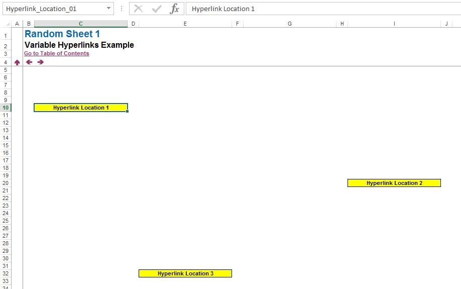
The other three locations are spread across two further worksheets.
Firstly, for reasons explained above, the six locations should be given range names, e.g. Hyperlink_Location_01 to Hyperlink_Location_06, say. Range names have previously been discussed in Naming Names.
Secondly, this model has a location selector:
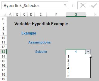
This has been created using a simple data validation list (please see >Data Validation for further details) and was named Hyperlink_Selector.
Thirdly, the range name HL_Variable_Hyperlink was defined as:
=IF(Hyperlink_Selector=”",Hyperlink_Location_01,
CHOOSE(Hyperlink_Selector,
Hyperlink_Location_01,
Hyperlink_Location_02,
Hyperlink_Location_03,
Hyperlink_Location_04,
Hyperlink_Location_05,
Hyperlink_Location_06)).
The function CHOOSE was used to select the appropriate destination: this is entirely arbitrary. Functions such as INDEX, OFFSET or INDIRECT could have been used instead. Certain functions do not seem to work well here though. IFERROR has issues, for example. Instead, I have used an IF statement to determine the hyperlink location if no selection has been made.
Finally, all I have to do is create the hyperlink. Insert Hyperlink (CTRL + K) does not work here as the HL_Variable_Hyperlink is not recognised as a valid hyperlink:
Therefore, we have to resort to the following function:
HYPERLINK(link_location,[friendly_name]).
creates a hyperlink formulaically:
- link_location is the reference the hyperlink should link to. If range names are used, there is a special syntax required. The range name should be in inverted commas and be preceded by the # sign; and
- friendly_name is optional (this is why Excel displays this argument in square brackets). This is the text to be displayed by the hyperlink otherwise it will display the cell reference.
In this example, the formula
=HYPERLINK(“#HL_Variable_Hyperlink”,”Go to Selection”).
has then been typed into cell D18:
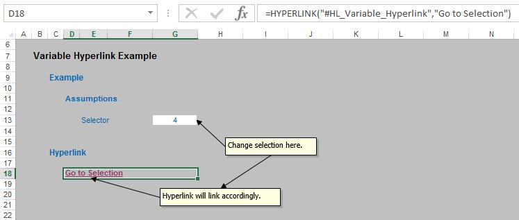
Now, if the selection is changed, the hyperlink will link as required. As mentioned above, please refer to the attached Excel file for an operating example.
Word to the Wise
The HYPERLINK function does not require the use of range names, but the syntax and formatting can be much more complex if range names are not used. The formula used in the example above is very simple to follow and it is for this reason that this particular technique is recommended.
As mentioned above, not all functions will work with HYPERLINK. It is not always clear why this may be. It is best trying to use HYPERLINK on a trial and error basis. However, it should be borne in mind that if the hyperlink reference is static, the Insert Hyperlink technique may be simpler in many instances.
If you have a query for this section, please feel free to drop Liam a line at liam.bastick@sumproduct.com or visit the website www.sumproduct.com

