Monday Morning Mulling: January 2025 Challenge

On the final Friday of each month, we set an Excel / Power Pivot / Power Query / Power BI problem for you to puzzle over for the weekend.  On the Monday, we publish a solution.  If you think there is an alternative answer, feel free to email us.  We’ll feel free to ignore you.

The Challenge

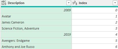
Last Friday’s challenge involved taking a list of movies with the released year, movie title, director’s name and genre, and unstacking it into a structured table.  Not all movies had genres allocated.

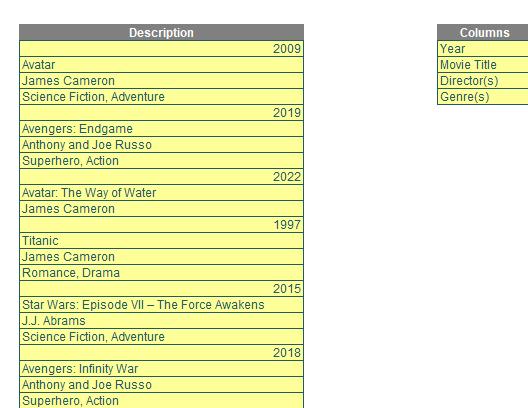
The single-column dataset (pictured in the top left of the image above) contained a mix of data points.  The challenge was to transform this chaotic dataset into a clean, structured table with clearly defined columns: Year, Movie Title, Director(s) and Genre(s).

The column headers needed to structure the data were provided in a separate table (pictured on the right side of the image).  Using these headers, the final goal was to create a tabular format, as illustrated in the final table at the bottom of the image.

Why was this important?  Inconsistent datasets like this frequently cropped up in the real world—ranging from survey results to logs or scraped data.  Without a clean structure, deriving insights or performing any meaningful analysis would have been next to impossible.

You can download the original question file here.

Remember, the solution had to adhere to the following:

• no VBA allowed; this is a Power Query challenge
• however, other solutions using Excel functions or Python in Excel were welcome!

The goal was to systematically extract and organise the data into structured columns for easier analysis and visualisation.

Suggested Solution

You can find our Excel file here, which shows our suggested solution.  The steps are detailed below.

Power Query Solution

The following steps outline how to resolve the challenge using Power Query, leveraging dynamic and reusable techniques to clean and restructure the data.

Firstly, we need to load the source data.  Select the ‘Movie Category’ table with the source data in a single column.  Click on any cell within the table, go to the Data tab in the Ribbon and click on ‘Get & Transform Data’.

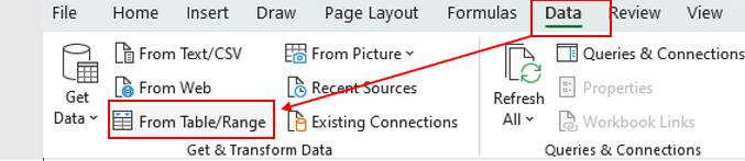
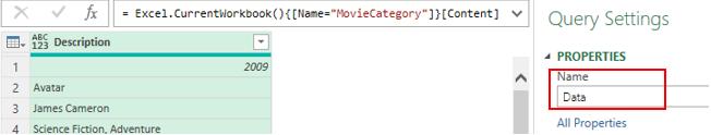
Select ‘From Table/Range’ to load the data into Power Query Editor.  The source data is loaded into Power Query from an Excel table named Data.

Secondly, we will add an Index column.  In the Power Query Ribbon, select Add Column -> Index Column.  Choose ‘From 0’ to start indexing at zero [0].

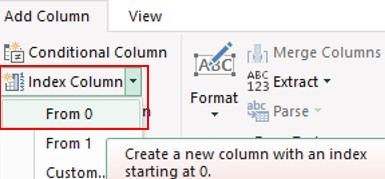
It should then look like the following screenshot: 

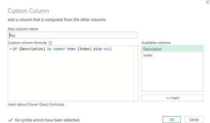
The next step is to generate keys to identify groups.  To define the starting point of each row or movie groups (e.g. one [1]  group per movie), we add a custom column by clicking Add Column -> Custom Column.  Please note that Power Query is case sensitive.  In the ‘Custom Column’ dialog, enter the column name as Key and then the M code as below:

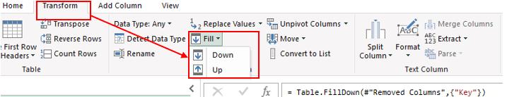
Then we need to fill down Key and remove unnecessary columns.  We can propagate the Key values downward to group all rows belonging to the same movie by selecting the Key column and going to the Transform tab and clicking on Fill -> Down.

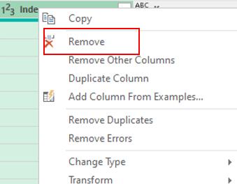
To simplify the data, we can select the Index column, right-click and choose Remove.

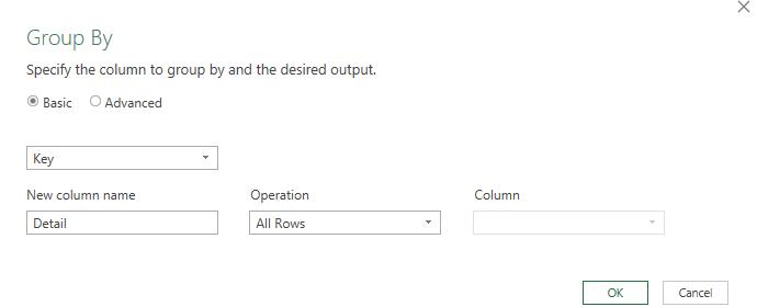
One crucial step in the process is grouping rows by Key.  To organise data by movie groups, we need to click on the Home tab and click on ‘Group By’.  In the dialog box, Group by Key, Operation should be ‘All Rows’ and name the new column Detail.

Then, click on the Formula bar, and transform the Table to a List by changing the following formula: 

to

The next step is to click the fx button next to the Formula bar to add a new step and transform nested tables into a single structured table by typing the formula:

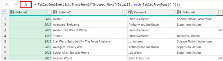
This step extracts each group and stacks rows into a flat table.  We are nearly there!  The last step is to rename columns.

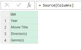
Load the separate TableCols table into Power Query and rename this table in Power Query to keep the same as TableCols.  To prepare the table for dynamic renaming, add a step using this formula:

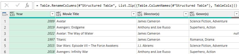
Go back to the Data and apply the renaming step:

After completing the steps, refresh the queries to ensure all changes are applied, then click 'Close & Load'.

We appreciate there are many, many ways this could have been achieved.  If you have produced an alternative, radically different approach, congratulations – that’s half the fun of Excel!

The Final Friday Fix will return on Friday 28 February 2025 with a new Excel Challenge.  In the meantime, please look out for the Daily Excel Tip on our home page and watch out for a new blog every business working day.